Chapter 7/16: Collection and Analysis of Rate Data
Polymath Tutorial
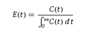
This is a tutorial to use the Polymath Regression tool to fit experimental tracer concentration data from a reactor to a polynomial C(t) = a0 + a1t + a2t2 + a3t3 + a4t4. Once we have C(t) we find the residence time distribution function E(t).
We will solve Example 16.2 in this tutorial.
This is our data set:
| t | 0 | 0.5 | 1 | 2 | 3 | 4 | 5 | 6 | 7 | 8 | 9 | 10 | 12 | 14 |
| C(t) | 0 | 0.6 | 1.4 | 5 | 8 | 10 | 8 | 6 | 4 | 3 | 2.2 | 1.6 | 0.6 | 0 |
We will split our data into two parts, an increasing and a decreasing part, and regress both the data sets separately.
Split the data at its maximum, and that happens at t = 4, when C(t) is 10. Our data now looks like this:
| t | 0 | 0.5 | 1 | 2 | 3 | 4 |
| C(t) | 0 | 0.6 | 1.4 | 5 | 8 | 10 |
and
| t | 4 | 5 | 6 | 7 | 8 | 9 | 10 | 12 | 14 |
| C(t) | 10 | 8 | 6 | 4 | 3 | 2.2 | 1.6 | 0.6 | 0 |
We will work with the first part in this tutorial.
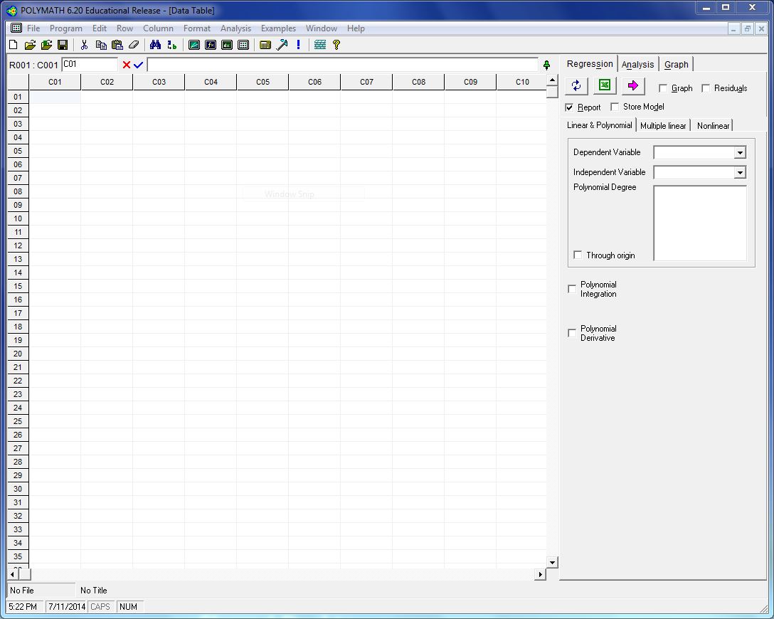
First, open Polymath and click on the Regression button on the toolbar ( ).
You should get a screen like this:
).
You should get a screen like this:
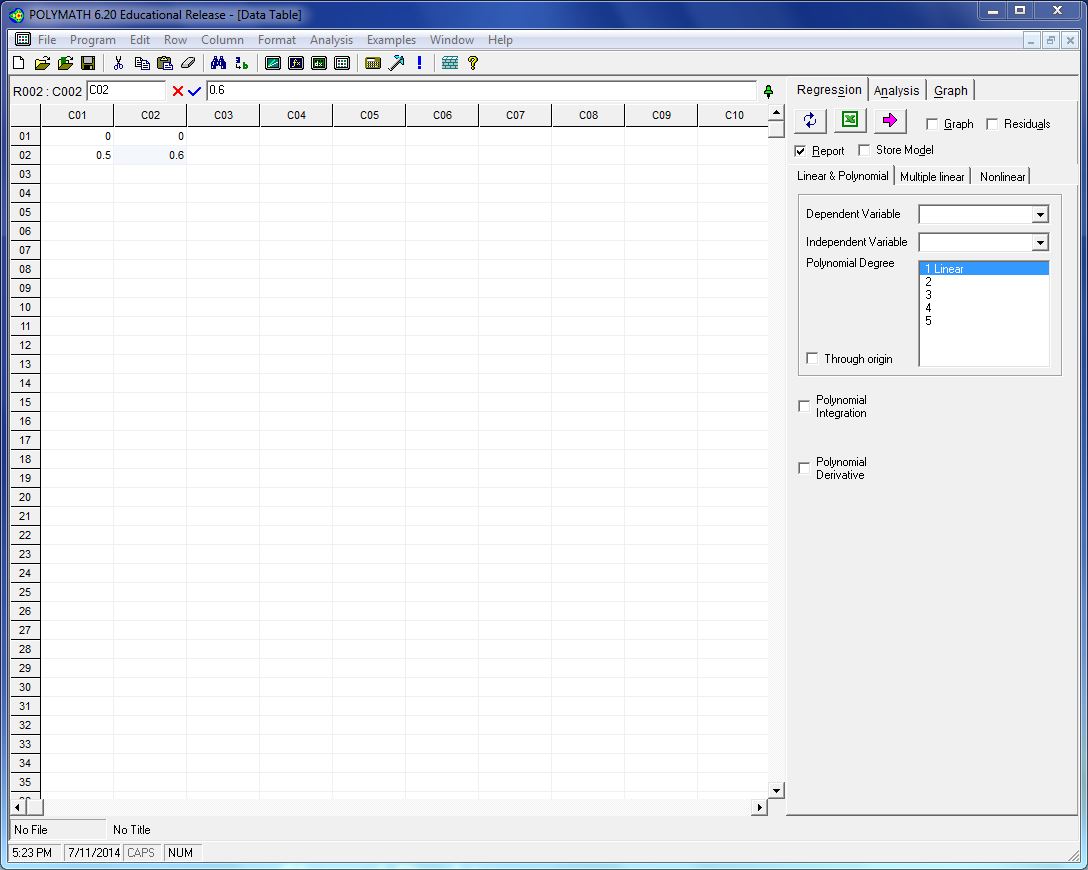
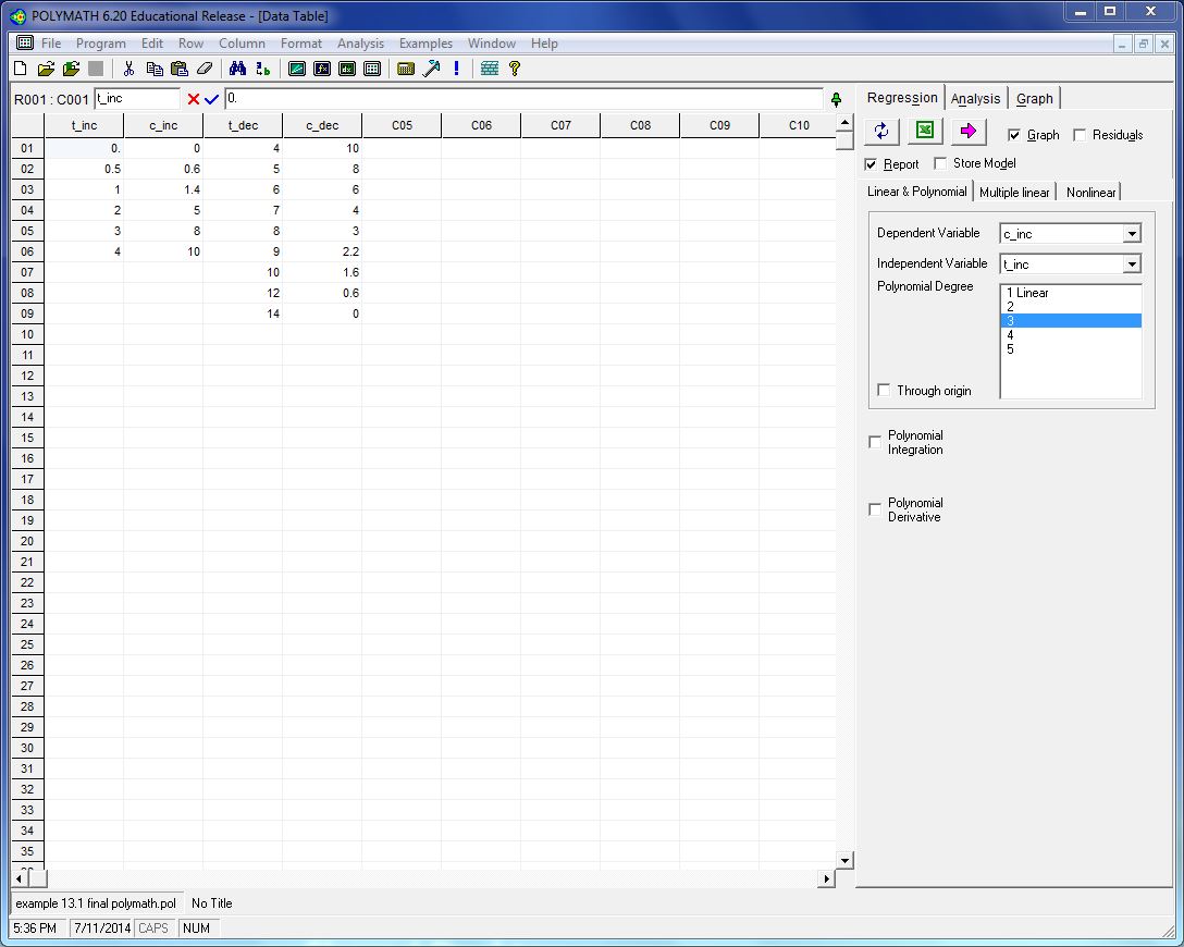
Input your data to be analyzed into the spreadsheet. It should look like this:
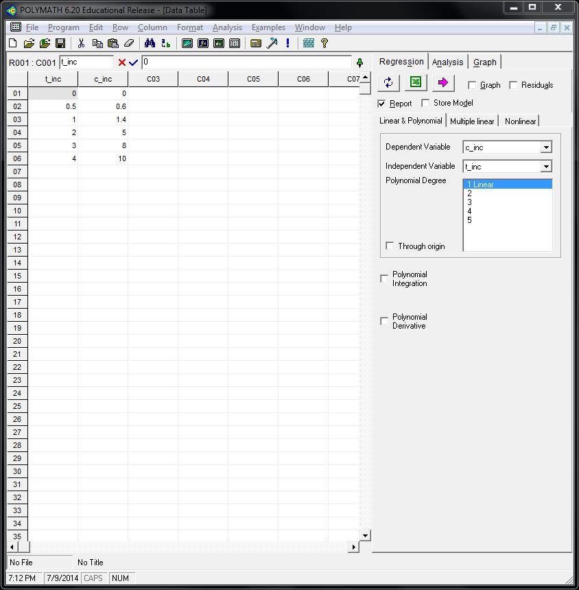
After entering the data to be analyzed, double-click on the C01 box to open a dialogue box to rename that column as “t_inc”, signifying the time of the increasing region of our data. Also rename C02 as “c_inc”. Now click on the Regression tab on the right side of the window, and select the "Linear and Polynomial" regression tab under the "Report" and "Store Model" check boxes. Clicking the refresh button on the left of the green excel sign updates the file. The window should look like this:
We now choose the independent variable as t_inc and the dependent variable as c_inc. After that, we choose the degree of our polynomial function that we want. Let us choose 3 for the purpose of this tutorial. We can also choose whether or not we want our fitted curve to pass through the origin. Check the “Graph” and the “Report” checkboxes to output them respectively. The screen now looks like this:

Clicking on the pink arrow will solve the system. You will see two new windows like this:
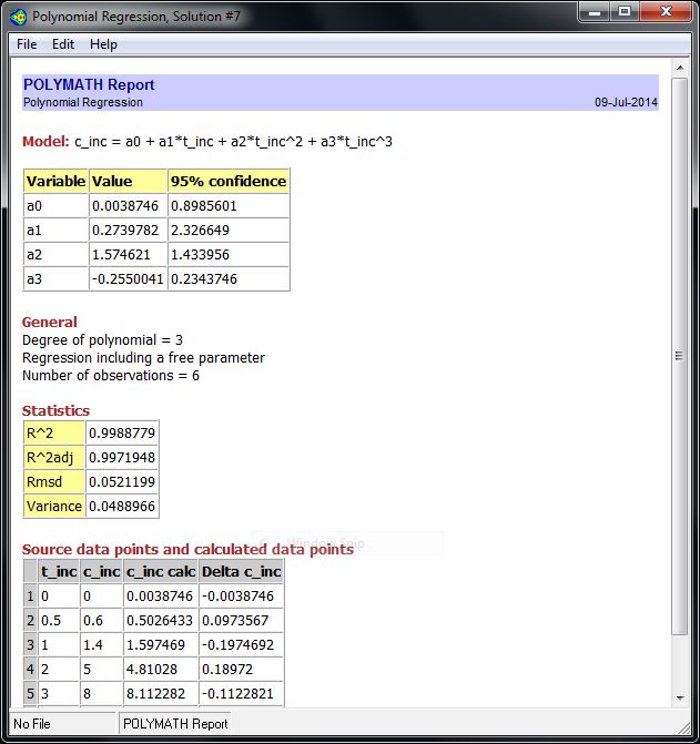
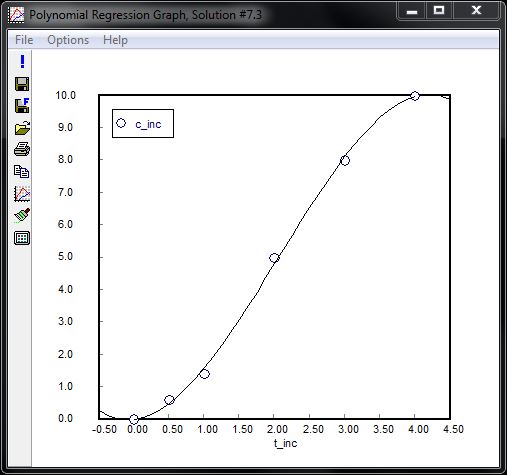
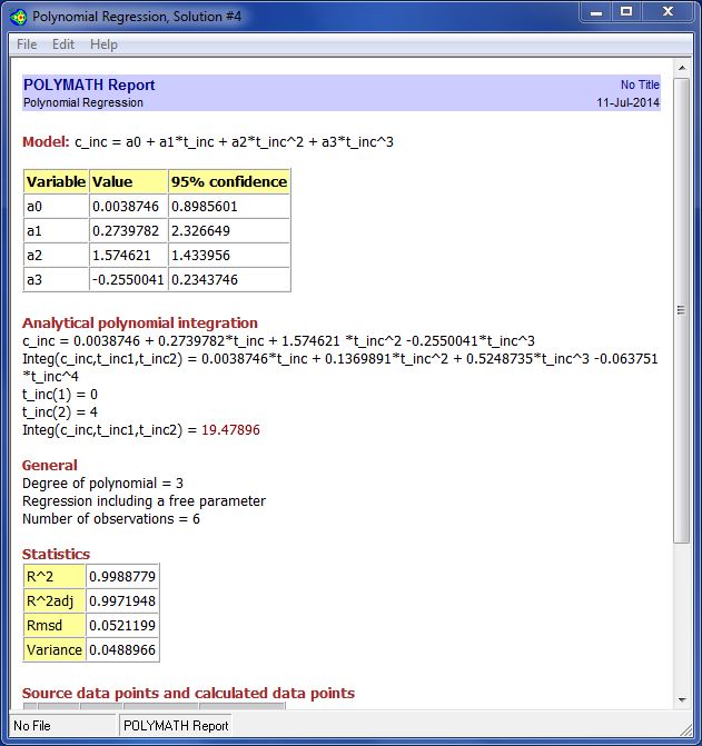
The report includes the model, the values of the model parameters, the statistical confidence of the parameters, and several other statistics. The graph shows the model that we fit to the data.
Hence, the best fit 3rd order polynomial is:
The Polymath window after the second part of the data is entered would look like this:
For regressing this data we regress using a 6th Order polynomial. Since a 6th Order polynomial is not available in “Linear and Polynomial” tab, we go to the “Nonlinear” tab and input our model:
c_dec = a0 + a1*t_dec + a2*t_dec^2 + a3*t_dec^3 + a4*t_dec^4 + a5*t_dec^5 + a6*t_dec^6
Where c_dec and t_dec are the concentration and time of the decreasing region of our data respectively.
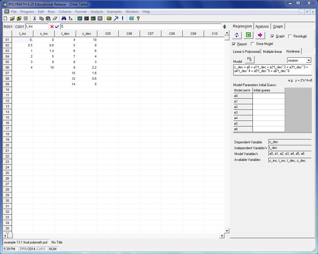
We also put in the initial guesses for our defined parameters a0 through a6, and use the mrqmin routine to regress our data.
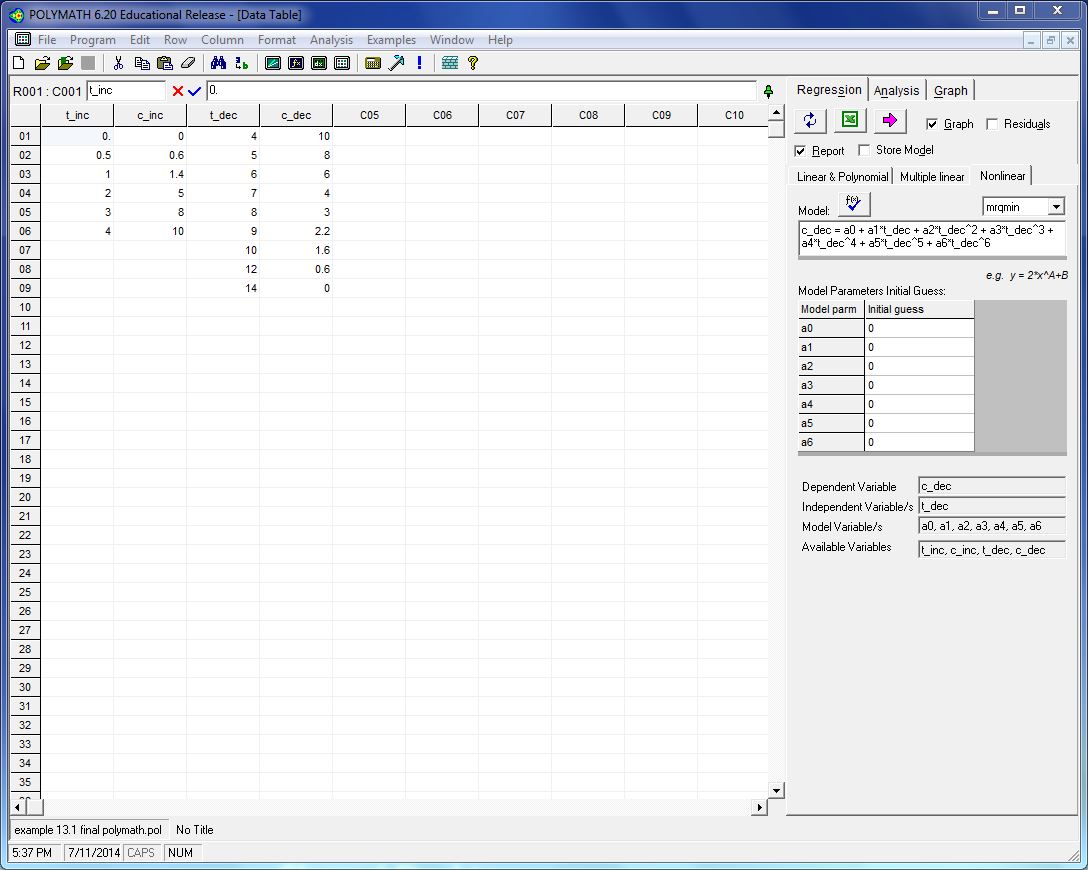
We now know that our model is ready for evaluation by looking at the blue tick in the f(x) command box. Pressing the pink arrow solves the program. The report and graph look like this:
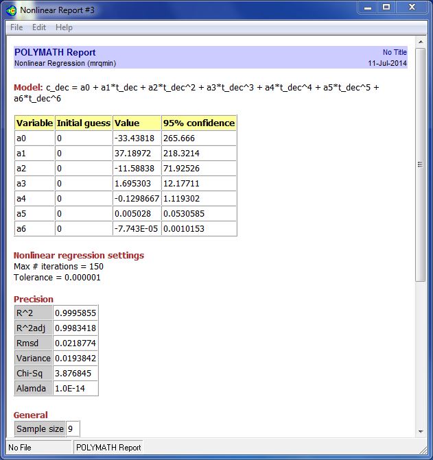
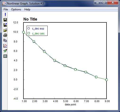
Hence the 6th order polynomial that fits the data best is
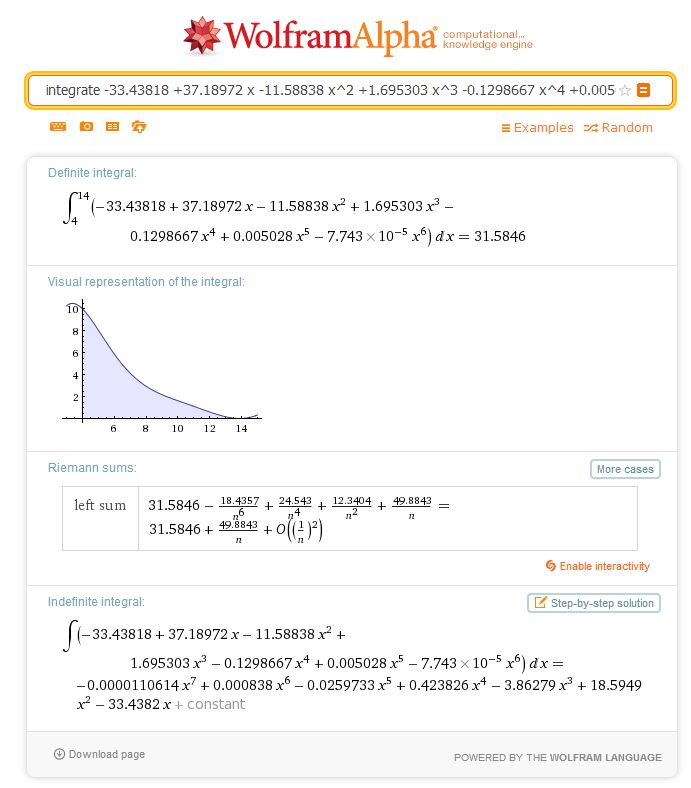
c_dec = -33.43818 + 37.18972*t_dec – 11.58838*t_dec^2 + 1.695303*t_dec^3 – 0.1298667*t_dec^4 + 0.005028*t_dec^5 – 7.743*10^-5*t_dec^6
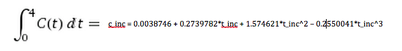
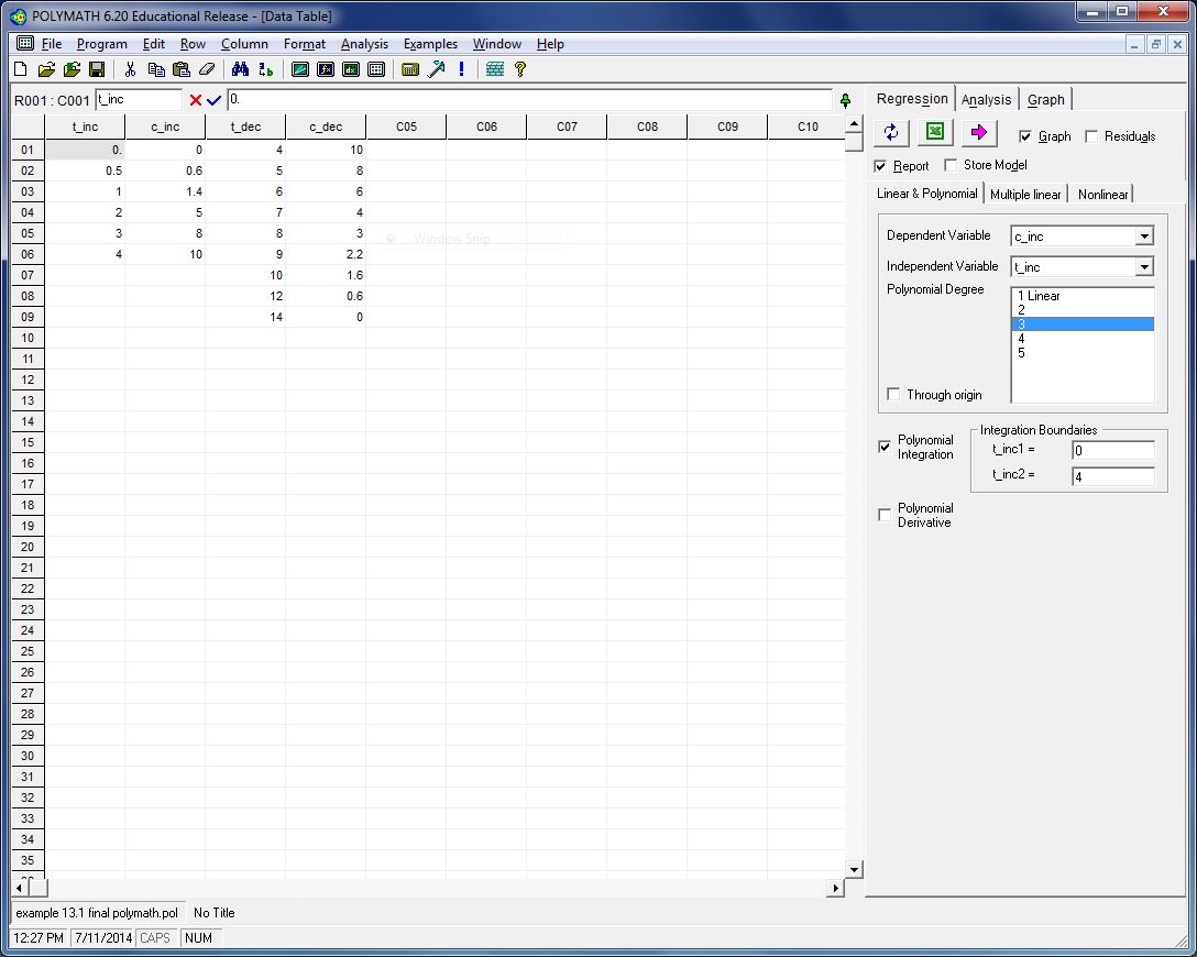
After we regress the data we find the area under the curve from t = 0 to 14. For the area under the increasing 3rd order polynomial, we can go back to the “Linear and Polynomial” tab, check the “Polynomial Integration” tab and set the boundaries as 0 and 4. The window looks like this:
When we run it, it gives out the integral in the report. The integral comes out to be 19.47896 as shown in the image:
For the non-linear 6th order model we must use some integration software to get the area under the curve. Wolframalpha.com gave the area to be 31.5846.
Now to get the E(t) curve we normalize the C(t) curve. The total area under the C(t) curve is 51.06356. Hence the E(t) curve would be given by E(t) = C(t)/51.06356 Thus,
E(t) = (0.0038746 + 0.2739782*t + 1.574621*t^2 – 0.2550041*t^3)/ 51.06356 for 0 ≤ t ≤ 4
And,
E(t) = (-33.43818 + 37.18972*t – 11.58838*t^2 + 1.695303*t^3 – 0.1298667*t^4 + 0.005028*t^5 – 7.743*10^-5*t^6)/51.06356 for 4 < t ≤ 14