I. Overview

            We start our section on tissue structure function with bone tissue. This is for two reasons: 1) from a mechanical standpoint, bone is historically the most studied tissue, and 2) due to 1) and the simpler behavior of bone compared to soft tissues, more is known about bone mechanics in relation to its structure. Bone is also a good starting point because it illustrates the principle of hierarchical structure function that is common to all biological tissues. In this section, we illustrate the anatomy and structure of bone tissue as the basis for studying tissue structure function and mechanically mediated tissue adaptation. We first begin by describing the hierarchical levels of bone structure (anatomy) and then describe how these levels are constructed by bone cells removing and adding matrix (physiology). We then discuss the linear elastic properties of bone and how the structure of bone (especially trabecular bone) has been related to its mechanical function as characterized by its constitutive models.

II.         Cortical Bone versus Trabecular Bone Structure

            Bone in human and other mammal bodies is generally classified into two types 1: Cortical bone, also known as compact bone and 2) Trabecular bone, also known as cancellous or spongy bone. These two types are classified as on the basis of porosity and the unit microstructure. Cortical bone is much denser with a porosity ranging between 5% and 10%.  Cortical bone is found primary is found in the shaft of long bones and forms the outer shell around cancellous bone at the end of joints and the vertebrae. A schematic showing a cortical shell around a generic long bone joint is shown below:                             

                       

 

The basic first level structure of cortical bone are osteons. Trabecular bone is much more porous with porosity ranging anywhere from 50% to 90%.   It is found in the end of long bones (see picture above), in vertebrae and in flat bones like the pelvis. Its basic first level structure is the trabeculae.

III.       Hierarchical Structure of Cortical Bone

            As with all biological tissues, cortical bone has a hierarchical structure. This means that cortical bone contains many different structures that exist on many levels of scale. The hierarchical organization of cortical bone is defined in the table below:

                                     Cortical Bone Structural Organization 

                        Level               Cortical Structure      Size Range                 h                                                ____________________________________________________

                        0                      Solid Material                > 3000 mm                   —

                        ____________________________________________________

                        1                      Secondary Osteons ^(A)  100 to 300 mm         < 0.1
                                                Primary Osteons ^(B)
                                                Plexiform (C)
                                                Interstitial Bone

                        ____________________________________________________

                        2                      Lamellae ^(A,B*,C*)     3 to 20 mm                < 0.1
                                                Lacunae ^(A,B,C,D)                 
                                                Cement Lines ^(A)

                        _____________________________________________________

                        3                      Collagen-                     0.06 to 0.6 mm         <0.1                                                                                Mineral                                    
                                                Composite  ^(A,B,C,D)

                        ^A - denotes structures found in secondary cortical bone
                               ^B - denotes structures found in primary lamellar cortical bone
                        ^C - denotes structures found in plexiform bone
                               ^D - denotes structures found in woven bone
                       * - indicates that structures are present in b and c, but much less than in a

                Table 1.      Cortical bone structural organization along with approximate physical scales.
                                   The parameter h is a ratio between the level i and the next most macroscopic level i - 1.
                                   This parameter is used in RVE analysis.

 

There are two reasons for numbering different levels of microstructural organization.  First, it provides a consistent way to compare different tissues. Second, it provides a consistent scheme for defining analysis levels for computational analysis of tissue micromechanics.  This numbering scheme will later be used to define analysis levels for RVE based analysis of cortical bone microstructure.  The 1st and 2nd organization levels reflect the fact that different types of cortical bone exist for both different species and different ages of different species.  Note that at the most basic or third level, all bone, to our current understanding, is composed of a type I collagen fiber-mineral composite.  Conversely, all bone tissue for the purpose of classic continuum analyses is considered to be a solid material with effective stiffness at the 0th structure.  In other words, a finite element analysis at the whole bone level would consider all cortical bone to be a solid material.

            Different types of cortical bone can first be differentiated at the first level structure.  However, different types of first level structures may still contain common second level entities such as lacunae and lamellae.  We next describe the different types of 1st level structure based on the text by Martin and Burr (1989).  As you will see, the different structural organizations at this level are usually associated with either a specific age, species, or both.

III.1       First Level Cortical Bone Structure

            As discussed by Martin and Burr (1989), there are four types of different organizations at what we have described as the 1^st structural level.  These four types of structure are called woven bone, primary bone, plexiform bone, and secondary bone. A general view of cortical bone structure showing some of the 1st and 2nd level structures is shown below:

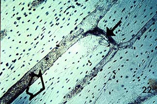
III.1.1    Woven-fibered cortical bone

            Woven cortical bone is better defined at the 1st structural level by what it lacks rather than by what it contains.  For instance, woven bone does not contain osteons as does primary and secondary bone, nor does it contain the brick-like structure of plexiform bone (Fig. 1).  Woven bone is thus the most disorganized of bone tissue owing to the circumstances in which it is formed.  Woven bone tissue is the only type of bone tissue which can be formed de novo, in other words it does not need to form on existing bone or cartilage tissue.  Woven bone tissue is often found in very young growing skeletons under the age of 5.  It is only found in the adult skeleton in cases of trauma or disease, most frequently occurring around bone fracture sites.  Woven bone is essentially an SOS response by the body to place a mechanically stiff structure within a needy area in a short period of time.  As such, woven bone is laid down very rapidly which explains its disorganized structure.  It generally contains more osteocytes (bone cells) than other types of bone tissue.  Woven bone is believed to be less dense because of the loose and disorganized packing of the type I collagen fibers (Martin and Burr, 1989).  It can become highly mineralized however, which may make it somewhat more brittle than other cortical bone tissue with different level one organization.  Very little is known, however, about the mechanical properties of woven bone tissue.  Christel et al., (1981) suggested that woven bone is less stiff than other types of bone tissue based on the premise that fracture callus is composed mainly of woven bone and is much less stiff than normal bone tissue.  Direct measurements of woven bone tissue stiffness have not been made.

III.1.2    Plexiform Cortical Bone Tissue

            Like woven bone, plexiform bone is formed more rapidly than primary or secondary lamellar bone tissue.  However, unlike woven bone, plexiform bone must offer increased mechanical support for longer periods of time.  Because of this, plexiform bone is primarily found in large rapidly growing animals such as cows or sheep.  Plexiform bone is rarely seen in humans.  Plexiform bone obtained its name from the vascular plexuses contained within lamellar bone sandwiched by nonlamellar bone (Martin and Burr, 1989).  In the figure below from Martin and Burr lamellar bone is shown on the top while woven bone is shown on the bottom:

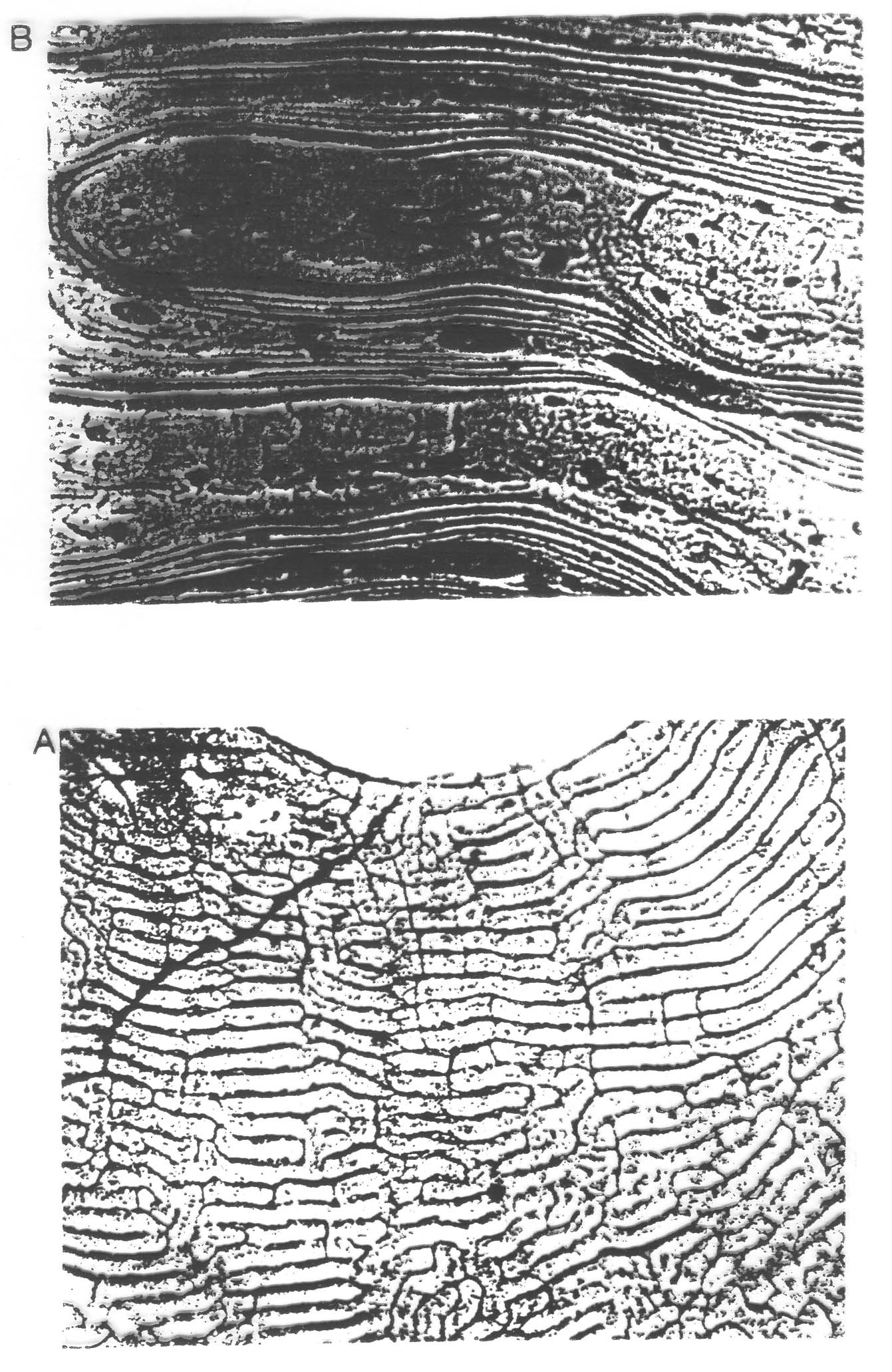
Plexiform bone arises from mineral buds which grow first perpendicular and then parallel to the outer bone surface.  This growing pattern produces the brick like structure characteristic of plexiform bone.  Each "brick" in plexiform bone is about 125 microns (mm) across (Martin and Burr, 1989).  Plexiform bone, like primary and secondary bone, must be formed on existing bone or cartilage surfaces and cannot be formed de novo like woven bone.  Because of its organization, plexiform bone offers much more surface area compared to primary or secondary bone upon which bone can be formed.  This increases the amount of bone which can be formed in a given time frame and provided a way to more rapidly increase bone stiffness and strength in a short period of time.  While plexiform may have greater stiffness than primary or secondary cortical bone, it may lack the crack arresting properties which would make it more suitable for more active species like canines (dogs) and humans.

III.1.3    Primary Osteonal Cortical Bone Tissue

            When bone tissue contains blood vessels surrounded by concentric rings of bone tissue it is called osteonal bone.  The structure including the central blood vessel and surrounding concentric bone tissue is called an osteon.  What differentiates primary from secondary osteonal cortical bone is the way in which the osteon is formed and the resulting differences in the 2^nd level structure.  Primary osteons are likely formed by mineralization of cartilage, thus being formed where bone was not present.  As such, they do not contain as many lamellae as secondary osteons.  Also, the vascular channels within primary osteons tend to be smaller than secondary osteons.  For this reason, Martin and Burr (1989) hypothesized that primary osteonal cortical bone may be mechanically stronger than secondary osteonal cortical bone.

III.1.4    Secondary Osteonal Cortical Bone Tissue

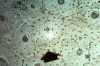
            Secondary osteons differ from primary osteons in that secondary osteons are formed by replacement of existing bone.  Secondary bone results from a process known as remodeling.  In remodeling, bone cells known as osteoclasts first resorb or eat away a section of bone in a tunnel called a cutting cone.  Following the osteoclasts are bone cells known as osteoblasts which then form bone to fill up the tunnel.  The osteoblasts fill up the tunnel in staggered amounts creating lamellae which exist at the 2^nd level of structure.  The osteoblasts do not completely fill the cutting cone but leave a center portion open.  This central portion is called a haversian canal (see cortical bone schematic).  The total diameter of a secondary osteon ranges from 200 to 300 microns (denoted as mm; equal to 0.2 to 0.3 millimeters).  In addition to osteons, secondary cortical bone tissue also contains interstitial bone, as shown in the cortical bone schematic. A histologic view of compact bone (from http://www.vms.hr/vms/atl/a_hist/ah062.htm) is seen below:

                                               

Some other pictures of compact bone histology may be viewed at http://www.grad.ttuhsc.edu/courses/histo/cartbone/intro.html, such as the histology section of cortical bone shown below:

                                    

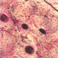
showing another cross section of osteonal cortical bone, and the following longitudinal section shown below:

                                      

Notice the haversian canals (large dark circles) and the rings of lamellae that surround them to form an osteon. The smaller dark circles are lacunar spaces within the bone.

.  The haversian canal in the center of the osteon has a diameter ranging between 50 to 90 mm.  Within the haversian canal is a blood vessel typically 15 mm in diameter (Martin and Burr, 1989).  Since nutrients which are necessary to keep cells and tissues alive can diffuse a limited distance through mineralized tissue, these blood vessels are necessary for bringing nutrients within a reasonable distance (about 150 mm) of osteocytes or bone cells which exist interior to the bone tissue.  In addition to blood vessels, haversian canals contain nerve fibers and other bone cells called bone lining cells.  Bone lining cells are actually osteoblasts which have taken on a different shape following the period in which they have formed bone.

III.2       Second Level Cortical Bone Structure

            The second level cortical bone structure consists of those entities which make up the osteons in primary and secondary bone and the "bricks" in plexiform bone.  Woven bone is again distinguished by the fact that no discernible entities exist at the second structural level.  Within osteonal (primary and secondary) and plexiform bone the four major matrix 2^nd level structural entities are lamellae, osteocyte lacunae, osteocyte canaliculi, and cement lines.  Lamellae are bands or layers of bone generally between 3 and 7 mm in thickness.  The lamellae are arranged concentrically around the central haversian canal in osteonal bone.  In plexiform bone the lamellae are sandwiched in between nonlamellar bone layers.  The lamellae in osteonal bone are separated by thin interlamellar layers in which the orientation of bone mineral may be altered.  Lamellae contain type I collagen fibers and mineral. 

            The osteocyte lacunae and canaliculi are actually holes within the bone matrix that contain bone cells called osteocytes and their processes.  Osteocytes evolve from osteoblasts which become entrapped in bone matrix during the mineralization process.  As such, the size of osteocyte lacunae if related to the original size of the osteoblast from which the osteocyte evolved.  Osteocyte lacunae have ellipsoidal shapes.  The maximum diameter of the lacunae generally ranges between about 10 to 20 mm.  Within the lacunae, the osteocytes sit within extracellular fluid.  Canaliculi are small tunnels which connect one lacunae to another lacunae.  Canalicular processes starting at osteocytes travel through the osteocytes canaliculi to connect osteocytes.  Many people believe that these interconnections provide a pathway through which osteocytes can communicate information about deformation states and thus in some way coordinate bone adaptation. A color view of 2nd level cortical bone structure is shown below (this picture was posted on the website http://medocs.ucdavis.edu/CHA/402/studyset/lab5/lab5.htm, which has a good collection of bone and cartilage histology):

            One of the most intriguing 2^nd level structural entities from a mechanical point of view is the cement line.  Cement lines are only found in secondary bone because they are the result of a remodeling process by which osteoclasts first resorb bone followed by osteoblasts forming bone.  The cement line occurs at the point bone resorption ends and bone formation begins.  Cement lines are about 1 to 5 microns in thickness.  Cement lines are believed to be type I collagen deficient structures.  Beyond this, the nature of cement has been widely debated.  Schaffler et al. (1987) found that cement lines were less mineralized than the surrounding bone tissue.  Many people have suggested that cement lines may serve to arrest crack growth in bone being that they are very compliant and likely to absorb energy.

III.3       Third Level Cortical Bone Structure

            The farther down the hierarchy of cortical bone structure we go, the more sketchy and less quantitative the information.  This is because it becomes more difficult to measure both bone structure and mechanics at increasingly small levels.  Most information about third level cortical bone structure mechanics is based on some quantitative measurements mixed with a great deal more theory.

            Third level cortical bone structure may be separated into two basic types, lamellar and woven.  Each type contains the basic type I collagen fiber/mineral composite.  What differentiates these two structures is how the composite, primarily the collagen fibers are organized.  In woven bone, the collagen fibers are randomly organized and very loosely packed.  A picture of woven bone forming at a fracture from the website http://www.pathguy.com/lectures/bones.htm is shown below:

             

As noted earlier, this results from the rapid manner in which bone is laid down.  Lamellar bone, which is found in plexiform, primary osteonal, and secondary osteonal bone, is laid down in a more organized fashion (as seen in the picture above) and constrasts very clearly to the woven bone above..  Although there is probably some continuum of structure between woven and lamellar bone, both bone structure is most frequently organized into these two categories.  The structure of lamellar bone is still widely debated, so we will discuss here the competing theories

III.3.1  Intra and Inter-Lamellar Type I Collagen Orientation

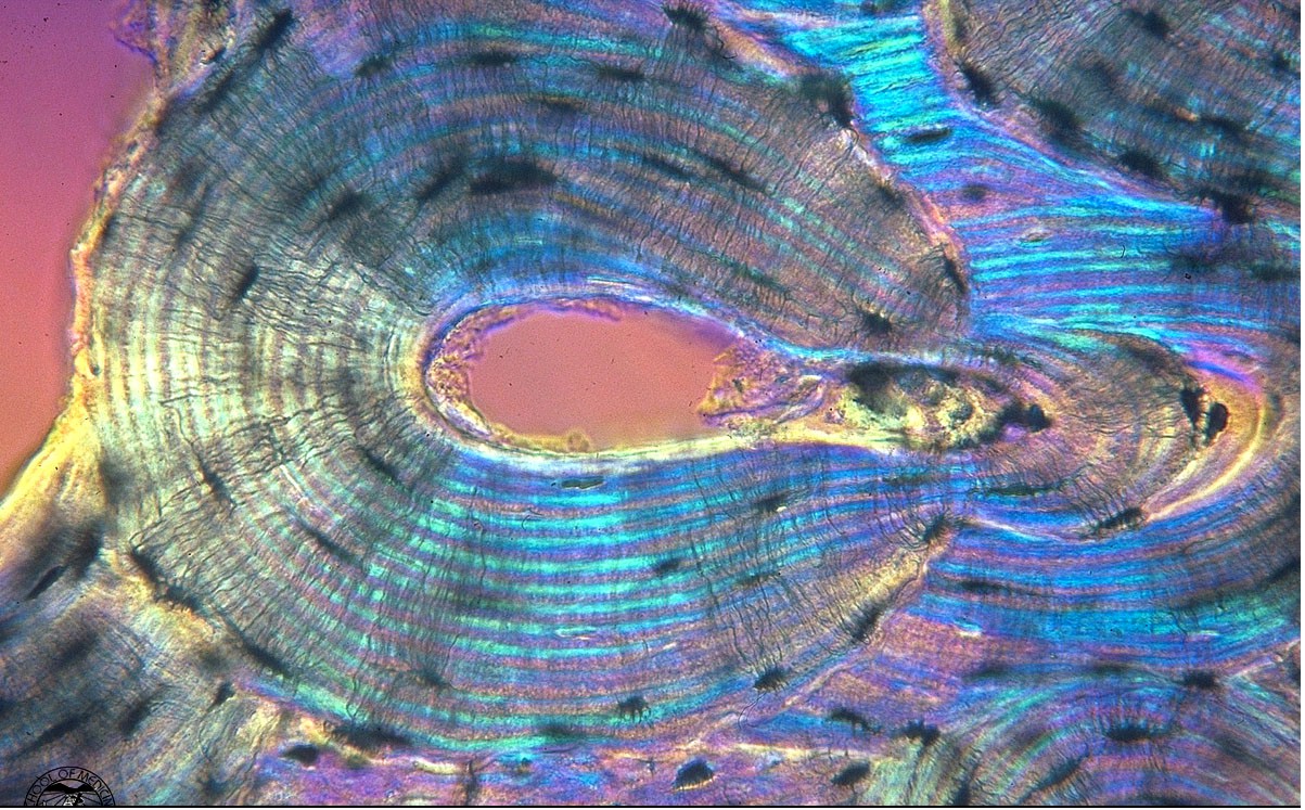
            One of the earliest theories to gain acceptance will be denoted here as the parallel collagen fiber orientation theory.  This is based largely on the work of Ascenzi and Bonucci (1970, 1976).  This theory suggests that collagen fibers within the same lamella are predominantly parallel to one another and have a preferred orientation within the lamellae.  The orientation of collagen fibers between lamellae may change up to 90^o in adjacent lamellae.  Based on this, three types of osteons containing three different type of lamellar sub-structures have been defined as drawn in Martin et al. 1998:

.  In the figure above, a is Type T, b is Type A, and c is Type L. Type L osteons are defined because there lamellae contain collagen fibers which are oriented perpendicular to the plane of the section, or parallel to the osteon axis.  These type of osteons appear dark under polarized light.  Type A osteons contain alternating fiber bundle orientations and thus give an alternating light and dark pattern under polarized light.  Finally, type T osteons contain lamellae with fiber bundles that are oriented parallel to the plane of the section.  With respect to the osteon axis, these bundles are oriented in a transverse spiral or circumferential hoop perpendicular to the center of the osteon.

            Giraud-Guille (1988) presented the twisted and orthogonal plywood model of collagen fibril orientation within cortical bone lamellae.  Giraud-Guille noted that the twisted plywood model as shown in Martin et al., 1998:

allows for parallel collagen fibrils which continuously rotate by a constant angle from plane to plane in a helical structure.  Another schematic of the twisted plywood model from Martin et al. (1998) is shown below:

The orthogonal plywood model consists of collagen fibrils which are parallel in a given plane but unlike the twisted plywood fibrils do not rotate continuously from plane to plane.  Instead, the fibrils can only take on one of two directions which are out of phase 90^o with each other.  Giraud-Guille believed that the orthogonal plywood model most closely resembles the type L and type T osteons from Ascenzi's model while the twisted plywood model would most likely explain the type A or alternating osteons from Ascenzi's model.  However, instead of three distinct structures creating three different polarized light patterns there would now be only two.

            Whereas both Ascenzi and colleagues and Giraud-Guille proposed models of collagen orientation assuming parallel fibers, Marotti and Muglia (1988) proposed that collagen fibrils were not parallel to each other, but instead had random orientations.  The alternating dark and light patterns seen in polarized light Marotti and Muglia believed were not the product of changes in orientation but were rather the result of different packing densities of collagen fibrils.  They defined dense and loose packed lamella (shown in Martin et al., 1998):

.  The light bands in polarized light microscopy they attributed to the loosely packed lamellae while the dark bands could be attributed to the densely packed lamellae.  Marotti and Muglia that the dense and loose packed lamellar model corresponded better with how bone was formed.  They suggested that alternating collagen orientations would require that osteoblasts somehow rotate when they were laying down bone.   Their model would require that osteoblasts would lay down an intertwined mesh of collagen fibers, but the density with which osteoblasts would lay down collagen fibers would change.

III.4.2  Mineral Packing within Collagen Fibrils

            A very thorough review of bone structure (as thorough as possible) from the angstrom level (mineral crystal) to the micron level (lamellae) was recently presented by Weiner and Traub (1992).  In that work, Wiener and Traub reviewed mineral structure, the mineral collagen composite, and how the mineral collagen composite fit into lamellae.  Collagen fibers, with a typical length of 0.015 mm, or .000015 mm, and a length of 3 mm, or .003 mm, packed together form collagen fibrils.  Within the packing of the collagen fibers are distinct gaps sometimes called hole zones (Fig. 14).  The structure of these holes is currently the focus of some debate.  In one model, the holes are completely isolated from each other.  In another model, the holes are contiguous and together from a groove about 0.015 mm thick and .370 mm long.  Within these holes mineral crystals form.  The mineral crystals in final form are believed to be made from a carbonate apatite mineral called dahllite which may initially resemble an octacalcium crystal.  The octacalcium crystal naturally forms in plates.  These mineral plates are typically 0.25 by 0.5 mm in length and width and have a thickness of 0.02 to 0.03 mm. It is these plates which are packed into the type I collagen fibrils.  Because of the nature of the packing, the orientation of the collagen fibrils will determine the orientation of the mineral crystals.  One such model is provided by Weiner and Traub (shown in Martin et al., 1998):

              

IV.       Trabecular Bone Structure

            Trabecular bone is the second type of bone tissue in the body.  It fills the end of long bones and also makes up the majority of vertebral bodies.  As with cortical bone, we will organize trabecular bone structure according to physical scale size.

Trabecular Bone Structural Organization

            Level               Trabecular Structure       Size Range                 h

            ____________________________________________________________

            0                      Solid Material                     > 3000 mm                   —

            ____________________________________________________________

            1                      Secondary Trabeculae ^(A)    75 to 200 mm             < 0.1                                                                          
                                    Primary Trabeculae (B)
                                                 Trabecular Packets  (D)

            ____________________________________________________________

            2                      Lamellae(^A,B*)                    1 to 20 mm                  <0.1                                      
                                    Lacunae ^(A,B,C*)                  
                                    Cement Lines ^(A)
                                    Canaliculi

            ____________________________________________________________

            3                      Collagen-                                 0.06 to 0.4 mm     <0.1                                                                    Mineral                                    
                                     Composite^(A,B,C)

                        ^A - denotes structures found in secondary trabecular bone

                        ^B - denotes structures found in primary trabecular bone

                        ^C - denotes structures found in woven bone

                        ^D - trabecular packets fall in between the 1^st and 2^nd level scalewise

                             but we have classified them as first level structures.

                        * - indicates that structures are present in b and c, but much less than in a

Table 2.            Trabecular bone structural organization along with approximate physical scales.  The parameter h is a ratio between the level i and the next most macroscopic level i - 1.  This parameter is used in RVE analysis.

            The major difference between trabecular and cortical bone structure is found on the 1^st and 2^nd structural levels.  It should be noted that the 3^rd level of trabecular bone structure is the same (as far as we know) as cortical bone structure.  The major mechanical property differences (as far as we know) between trabecular and cortical bone are the effective stiffness of the 0^th and 1^st structural level.  Trabecular bone is more compliant than cortical bone and it is believe to distribute and dissipate the energy from articular contact loads.  Trabecular bone contributes about 20% of the total skeletal mass within the body while cortical bone contributes the remaining 80%.  However, trabecular bone has a much greater surface area than cortical bone.  Within the skeleton, trabecular bone has a total surface area of 7.0 x 10⁶ mm² while cortical bone has a total surface area of 3.5 x 10⁶ mm².  A comparison between the general features of cortical bone and trabecular bone including volume fraction and surface area is given below (Jee,1983):

Structural Feature                                 Cortical Bone                           Trabecular Bone

Volume Fraction                                   0.90 (0.85 - 0.95)                    0.20 (0.05 - 0.60)

(mm³/mm³)

Surface/Bone Volume                           2.5                                           20

(mm²/mm³)

Total Bone Volume                               1.4 x 10^⁶                                  0.35 x 10^⁶

(mm³)

Total Internal Surface                            3.5 x 10^⁶                                  7.0 x 10^⁶

(mm²)

Table 3.            Comparison of some structural features of cortical and trabecular bone.

IV.1       First Level Trabecular Bone Structure

            One of the biggest differences between trabecular and cortical bone is noticeable at the 1^st level structure.  As seen in the first table, trabecular bone is much more porous than cortical bone.  Trabecular bone may have bone volume fraction ranging from just over 5% to a maximum of 60%.  Bone volume fraction is defined as the volume of bone tissue (including internal pores like lacunae and canaliculi) per total volume.  The trabecular bone volume fraction varies between different bones, with age, and between species.  The basic structural entity at the first level of trabecular bone is the trabecula.  Trabecula are most often characterized as rod or plate like structures (as seen in these renderings from the website http://www.npaci.edu/envision/v15.3/keaveny.html). 

                                  

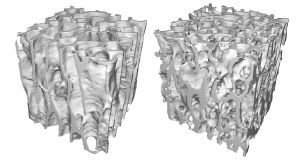
Early finite element models of 1^st level trabecular structure did indeed model trabeculae using plate and beam finite elements.  Trabecula are in general no greater than 200 mm in thickness and about 1000 mm or 1 mm long.  Unlike osteons, the basic structural unit of cortical bone, trabeculae in general do not have a central canal with a blood vessel.  (Note: we are characterizing the basic or 1st level structural unit of trabecular bone as the trabecula based on the fact that it has similar size ranges as the osteon.  Jee (1983) denotes the trabecular packet as the basic structural unit of trabecular bone based on the fact that it is the basic remodeling unit of trabecular bone just as the osteon is the basic remodeling unit of cortical bone).  In rare circumstances it is possible to find unusually thick trabeculae containing a blood vessel and some osteon like structure with concentric lamellae.

            Another structure found within the trabecula is the trabecular packet.  We have chosen to define the trabecular packet as a 1^st level structure because of its size.  The trabecular packet is only found in secondary trabecular bone because it is the product of bone remodeling in which bone cells called osteoclasts first remove bone and bone cells called osteoblasts then deposit new bone were the old bone was removed.  Trabecular bone can only be remodeled from the outer surface of trabeculae.  The typical trabecular packet has a crescent shape (Jee, 1983).  A typical trabecular packet is about 50 mm thick and about 1 mm long.  Trabecular packets contain lamellae and are attached to adjacent bone by cement lines similar to osteons in cortical bone.

IV.2       Second Level Trabecular Bone Structure

            The 2^nd level structure of trabecular bone has most of the same entities as the 2^nd level structure of cortical bone including lamellae, lacunae, canaliculi, and cement lines.  Trabecular bone, as noted before, does not generally contain vascular channels like cortical bone.  What differentiates trabecular bone from cortical bone structure is the arrangement and size of these entities.  For instance, although lamellae within trabecular bone structure are of approximately the same thickness as cortical bone (about 3 mm; Kragstrup et al., 1983), the arrangement of lamellae is different.  Lamellae are not arranged concentrically in trabecular bone as in cortical bone, but are rather arranged longitudinally along the trabeculae within trabecular packets (Fig. 5).  Krapstrup et al. noted that the thickness of lamellae tended to increase in age for females.  Cannoli et al. (1982) found a higher density and larger lacunae within metaphyseal and epiphyseal trabecular bone than in diaphyseal or metaphyseal cortical bone.  They found that the lacunae were ellipsoidal in both areas.  The cross-sectional area of lacunae in trabecular bone ranged between 50.6 and 53.8 mm² while the cross-sectional area of lacunae in cortical bone ranged between 35 and 26 mm².  Thus, the lamellar pattern as well as the lacunae size differ between trabecular and cortical bone.

IV.3       Third Level Trabecular Bone Structure

            The third level of trabecular bone structure consists of the same entities as the third level of cortical bone structure, namely the collagen fibril-mineral composite.  As no detailed studies have been perfomed on trabecular bone at this level, it is presumed for now that the structure at this level, i.e collagen fibril organization within lamellae and collagen-mineral structure, is the same as for cortical bone.

            In this section we discuss how various aspects of both cortical and trabecular bone structure as described in the previous section affect their function represented by the mechanical properties of stiffness and strength. It is very important to note that we may define material properties like stiffness and strength for each level of structure. For example, a section of cortical bone may have an elastic modulus just as an individual osteon may have an elastic modulus. The other critical note to make is that material properties at a more macroscopic level are a function both of material properties and the spatial arrangement or architecture of materials at the more microscopic level. This is the essence of tissue structure function. Thus, cortical bone stiffness, that is stiffness at the 0th level, is a function of osteon arrangement (spatial arrangement or architecture at the 1st level), the stiffness of individual osteons (material properties at the 1st level), the degree of mineralization of the osteons (spatial arrangement and materials properties at the 3rd level, etc. One goal of biomechanics is to determine how changes of a given structural level, due perhaps to disease or a conscious intervention to alter bone structure, affect the load carrying capacity of bone. This fits into the following feedback scenario:

                             

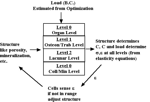
The load on the whole bone (determined for instance by the optimization analysis we discussed previously) generates stress and strain at each level of structure. The level of stress and strain generated by the load is a function of the hierarchical material properties. The subsequent stress or strain is sensed by the cell to determine if it is within acceptable limits, both lower and upper. If not, the cell can act on the matrix to alter the bone structure and thereby alter the mechanical properties. This changes (assuming the load stays the same) the stress and strain felt by the cell. The cells acting together are believed to regulate the bone structure in response to their mechanical environment. This in turn determines tissue stiffness and strength. Diseases that affect either the cells ability to sense mechanical stress or to alter bone matrix can lead to deficient mechanical properties. We next describe one aspect of the loop, namely how different aspects of bone structure affect mechanical properties, generally known as structure function relationshisps. We begin with a definition of stress, strain and constitutive properties viewed in a hierarchical perspective.

V.       Hierarchical Stress, Strain and Constitutive Properties

            Both cortical and trabecular bone have hierarchical structures, as do all biological tissues. Just as their are structural entities at different length scales from sub-micron to centimeter, so we can define mechanical behavior including stress, strain and material properties at each level of structure. For example, cortical bone properties are often determined by machining a tensile specimen from the cortical diaphysis. This specimen may have a gauge area of 5x5mm and a length of 5 mm. A schematic is shown below:

                                                

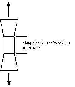
Stress in this gauge section is computed simply as the force from the load cell in tension divided by the cross sectional area of the gauge. Deformation is measured as the change in length of the gauge section divided by the original length of the gauge section. The gauge section, however, may contain many osteons. It is obvious that the experimental stress and strain are average over many osteons. This indicates that the stress we measure in the testing set-up above cannot represent the stress in a single osteon. We can relate the average stress (the 0th level structure in the cortical bone organizational chart) to the first level stress at the osteonal level using the following equation:

                       

where denotes effective stress  which is eqiuvalent to stress at the 0th level  in our cortical bone organizational chart,  denotes the volume of the cube of bone we are testing, which is equivalent to a volume at the first level of scale ,  denotes stress at the oseon level, which is equivalent to the 1st level stress  in the cortical bone organizational chart.  We can also write the same relationship for the average strain:

                        

where the levels are as in the average stress equation and e is strain.

Even though we can write strain and stress for a given macroscopic level as he average over the next microscopic level, we generally cannot do the same for the constitutive equations. This is because the constitutive properties vary over distinct phases of material at the microscopic level. For example, with cortical bone, the microstructure contains stiffness properties for the osteons and the blood vessel space, in addition to the interstitial bone. If we assume that there are n phases of microstructure, then when can write the constitutive equation for the effective or macroscopic level as:

        

We can rewrite the above equations condensed in matrix form as:

                         

where M is known as a strain localization matrix or local matrix for short. The form of M can vary depending on the assumed model (if we are doing computational or analytical models) or on the experimental measures used to quantify structure. What the above equations represents is what we know intuitively, namely that the effective properties at a macroscopic level depend on the microscopic properties [C], the the spatial arrangement or architecture of those microscopic properties [M]. It is important to note that the above equation governs the relationship between any structural level defined in the cortical and trabecular bone organization chart. That is, the effective properties of osteons may be related to the distribution of lacunae, the collagen organization, degree of mineralization, etc.

 For trabecular bone, mechanical properties at the 0th level, most commonly referred to as "effective" or "continuum" level trabecular bone properties, are determined experimentally most often by testing cubes of trabecular bone between 8mm and 1 cm on a side in compression, underneath a loading platen:

               

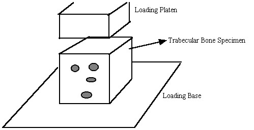
Again, as with cortical bone, It is assumed in these tests that one average stress measure can be computed as the force divided by the area of a face of the cube. Strain is computed by divided the change in length of the cube by the original length of the cube. It is important to note that by computing the stress this way we are computing an average or effective stress. In other words, the stress we compute is the same as if we average the stress over all the individual trabeculae and the available pore space. This can be written mathematically as:

                       

where denotes effective stress  which is eqiuvalent to stress at the 0th level  in our trabecular bone organizational chart,  denotes the volume of the cube we are testing, which is equivalent to a volume at the first level of scale ,  denotes stress at the trabecula level, which is equivalent to the 1st level stress  in the trabecular bone organizational chart.   The average strain is defined in the same manner as:

                     

where the superscripts and the levels are the same as defined for the average stress. The constitutive matrix at the effective level is related to the microscopic level properties using the same rule for the constitutive equation we used for cortical bone.

III         Elastic/Strength Properties of Cortical Bone at the 0th Level: Influence of 1st Level Structure

            Mechanical stiffness values have been measured most often for secondary haversian bone human and cow (bovine) bone as well as bovine plexiform bone.  Stiffness has been measured using both standard mechanical testing techniques as well as ultrasonic measurements where the velocity of waves propagating through a material is measured.  This wave velocity is related to the stiffness and the density of the material.

            Reilly et al. (1974) measured the stiffness of human secondary osteonal bone, bovine secondary haversian bone, and primary bovine bone.  Reilly et al. did not measure Hooke's constants directly, but rather made some measure of moduli in the inferior-superior direction (denoted the 33 direction in Hooke's Law) and the radial direction within the cross section of the long bone.  Reilly et al. found:

Bone Type                   Modulus I-S     Modulus Radial            Strength IST     Strenght Radial

Hum. Haversian            17.9 GPa         10.1 GPa                     135 MPa          53 MPa

Bovine Haversian          23.1 GPa         10.4 GPa                     150 MPa          49 MPa

Bovine Primary             26.5 GPa         11.0 GPa                     167 MPa          55 MPa

Note that bone stiffness is greater in the I-S direction along the osteonal length than in the transverse direction across the osteons.  Also note that secondary osteons (haversian bone) with more lamellae tend to reduce both the stiffness and strength of cortical bone.

            Katz et al. (1984) measured and compared the orthotropic elastic constants of bovine plexiform bone and human secondary bone:

            Elastic Constant            Plexiform Value            Secondary Value

            C₁₁₁₁                               22.4 GPa                     21.2 GPa

            C₂₂₂₂                               25.0 GPa                     21.0 GPa

            C₃₃₃₃                               35.0 GPa                     29.0 GPa

            C2323                               8.2 GPa                       6.3 GPa

            C1313                               7.1 GPa                       6.3 GPa

            C₁₂₁₂                               6.1 GPa                       5.4 GPa

            C₁₁₂₂                               14.0 GPa                     11.7 GPa

            C₂₂₃₃                               13.6 GPa                     11.1 GPa

            C₁₁₃₃                               15.8 GPa                     12.7 GPa

Notice that the plexiform bone with the brick like structure has orthotropic symmetry while the secondary haversian canal is nearly transversely isotropic.  The type of material symmetry present results from the different types of 1^st level structures.  Osteons are tube structures which exhibit a transversely isotropic symmetry while the brick like structures of plexiform bone exhibit an orthotropic symmetry depending on the aspect ratios of the brick.

An overview (or representative average) of cortical bone properties for human and bovine (cow) were presented by Martin et al. (1998):

Property                                        Human Value                            Bovine Value
Elastic Modulus Transverse            17.4 GPa                                 20.4 GPa
Elastic Modulus Long                     9.6 GPa                                   11.7 GPa
Shear Modulus                              3.5 GPa                                   4.1 GPa
Tensile Yield Stress Long               115 M Pa                               141 MPa
Tensile Ult Stress Long                   133 M Pa                               156 MPa
Tensile Ult Stress Trans                   51 M Pa                                50 MPa
Comp Yield Stress Long                182 M Pa                               196 MPa
Comp Yield Stress Trans               121 M Pa                               150 MPa
Comp Ult Stress Long                   195 M Pa                               237 MPa
Comp Ult Stress Trans                   133 M Pa                               178 MPa
Tensile Ultimate Strain                    2.9 - 3.2%                             .67 - .72%
Compressive Ult. Strain                  2.2 - 4.6%                             2.5 - 5.2%

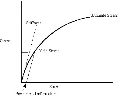
It is important to note what the quantities of yield and ultimate stress represent. Although bone is not an elastic-plastic material in the classic sense like metals, bone will yield. This means that under high enough loads, permanent deformation will occur in bone. The ultimate strength is the stress at which the bone undergoes catastrophic failure. The elastic modulus is the bone stiffness. We illustrate these concepts on a schematic stress strain curve below:

                         

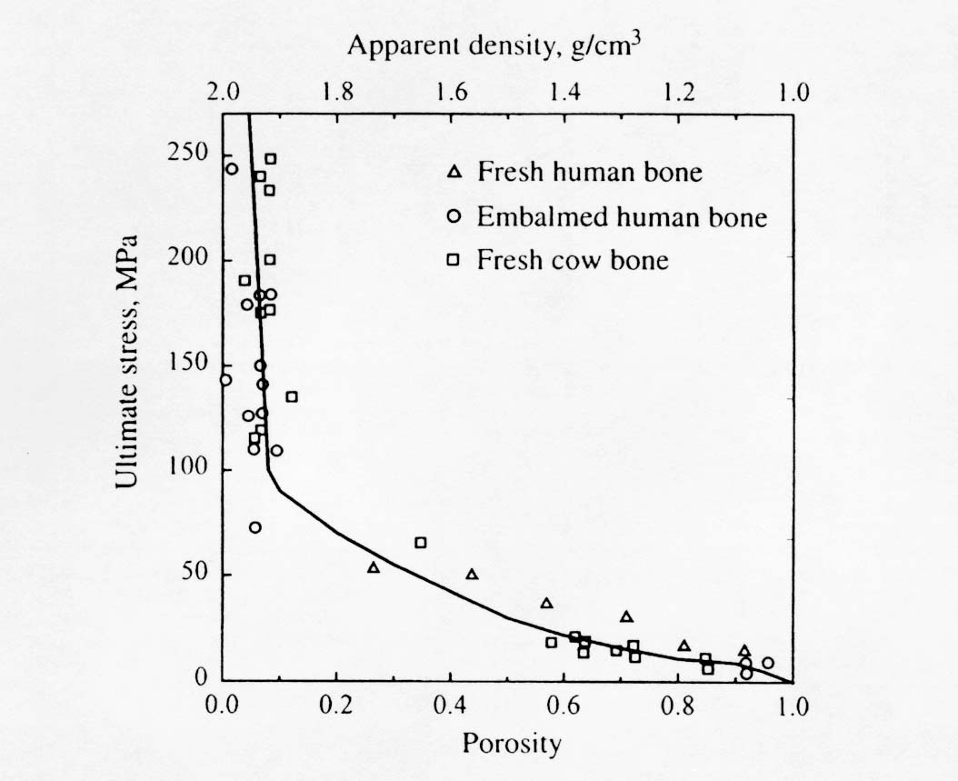
Porosity

            We saw that cortical bone properties are significantly affect be the microstructural differences between osteonal and plexiform bone. However, these bone structure function relationships were qualitative, due to difficulties in quantifying these types of microstructures. One microstructural variable that has a significant influence on bone mechanical properties is porosity. Porosity is difficult to classify however, because it occurs across multiple scales. In cortical bone, porosity may result from haversian canals and resorption cavities on the 1st level (~ 100 to 200 microns) down to lacunae and canaliculi at the 2nd level (~5 to 20 microns). In cortical bone, although porosity measurements take all these voids into account, it is believed that the larger scale voids, the haversian canals, have a large affect on mechanical properties.
Both Schaffler and Burr (1988) and Currey (1988) measured tensile elastic modulus of cortical bone and compared the results to measures of porosity. Both found statistically significant relationships and derived empirical relationships between porosity p and Young's modulus E:

                                     

Note that Young's modulus is given in GPa and that the exponent on porosity is very large and nonlinear. This means that the moment one introduces porosity into bone, there is a large decrease in stiffness. The effect of ultimate stress on porosity is similar. Martin et al. (1998) present a composite graph showing multiple experiments relating ultimate stress to porosity:

                                     

Mineralization

            A significant component of bone that differentiates it from soft tissues is the presence of the HA like ceramic mineral. It is postulated that the mineral component gives bone its high stiffness compared to soft tissues while the type I collagen contributes to the post-yield behavior of bone. Currey (1986) found that specific mineralization and porosity could explain 84% of the variance in cortical bone stiffness. Specific mineralization is defined as the volume of mineral per volume of bone matrix exclusive of voids. Schaffler and Burr (1988) found that mineral did explain some variance in cortical bone stiffness, but not a significant amount due to the fact that there was little variability in specific mineralization between specimens. They derived an equation relating mineral to elastic modulus:

                                     

Note that the exponent for mineralization is not as high for porosity, indicating that porosity has a large affect on bone stiffness than mineralization. This of course is only true if the variation in mineralization is small.

VI         Effect of 2nd Order Structure on 1st Order Material Properties

            Very little mechanical data is available on 2nd level cortical bone mechanics.  Ascenzi and colleagues (see Martin and Burr, 1998) have performed the most mechanical testing of individual osteons.  The procedure by which Ascenzi and co-workers have tested osteons is illustrated below:

                               

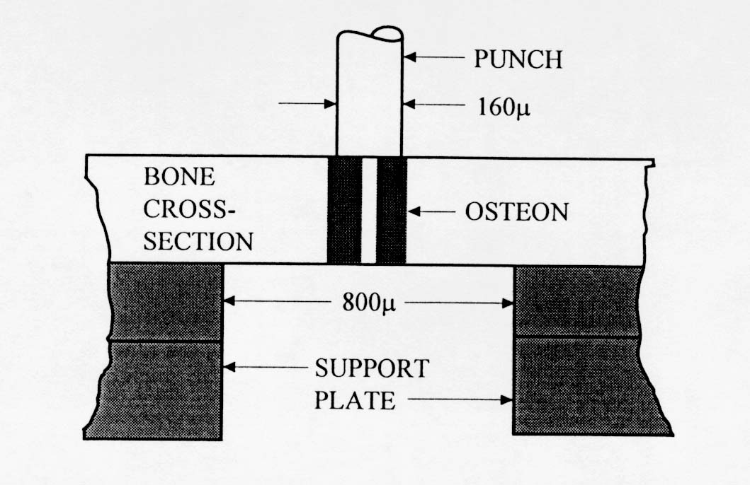
.  The results from Ascenzi's testing indicate that secondary osteon stiffness is less than that of large cortical bone specimens.  This would indicate that some other structures in cortical bone, perhaps interstitial bone, contribute more to the overall stiffness of cortical bone.

Osteon Properties from Ascenzi

Osteon type                    Mechanical Test         Elastic Modulus(GPa)            Ultimate Stress (MPa)

Longitudinal                  Compression                6.3                                           110

Transverse                    Compression                9.3                                           164

Alternating                    Compression                7.4                                           134

Longitudinal                  Tension                        11.7                                         114

Alternating                    Tension                        5.5                                           94

Longitudinal                  Shear                           3.3                                           46

Transverse                    Shear                           4.2                                           57

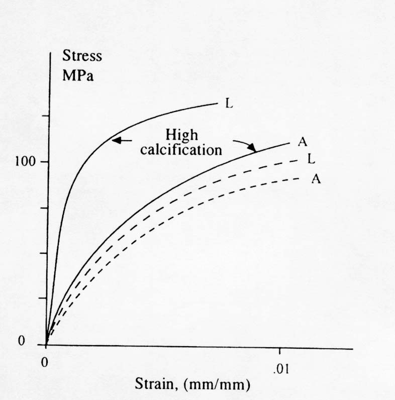
Alternating                    Shear                           4.1                                           55

The terms longitudinal and alternating refer to how the collagen fiber bundles are oriented with respect to the plane of the osteon section.  Notice that collagen fiber bundles oriented with the direction of testing produce a higher normal stiffness while collagen fiber bundles oriented out of the plane of testing produce a lower normal stiffness but a higher shear stiffness. Ascenzi also reported the affect of mineralization on the properties of these different types of osteons. The effect is illustrated in the stress strain diagram below:

            Another important aspect of how 2^nd level structure affects cortical bone mechanics is crack propagation and fatigue life.  Since it seems that both primary and plexiform bone have higher strength and stiffness than secondary osteonal bone, the question arises as to why humans and other active mammals have secondary bone rather than plexiform or primary bone.  Although there may be many metabolic reasons, one mechanical reason has to do with crack initiation and arrest.  Since humans and other smaller mammals are much more active than cows and sheep, their bones are subject to many cycles of loading.  This would make human bone much more subject to fatigue failure.  Once mechanical advantage of secondary bone is that it has many compliant interfaces such as cement lines.  These weak interfaces provide many opportunities for crack arrest , thus making secondary osteonal bone perhaps more fatigue resistant.

VII.         Dependence of Trabecular Bone Effective (0th Level) Properties on 1st Level Structure: Part I Quantifying Trabecular Structure

            The main features of trabecular bone structure at the 1st level are the high porosity and the intricate architecture and orientation of the complicated rod and plate structure of trabeculae. We can expect therefore that these features along with mineralization to be the major factors contributing to the effective stiffness of trabecular bone. This is similar to the determinants of cortical bone effective stiffness, which were osteons versus plexiform structure, the amount of porosity and the degree of mineralization. However, a significant difference between cortical bone 1st level structure and trabecular bone 1st level structure is the substantial variation in 1st level trabecular bone structure compared to cortical bone structure. Whereas most human adult structure is osteonal we a tight porosity range of 5 to 10%, human adult trabecular bone has a much larger range of porosity (10 to 50%) and a much more varied architecture. Osteons by and large have fairly consistent orientation in cortical bone but rods and plates in trabecular bone have a much greater variation in orientation. Therefore in addition to quantifying porosity in trabecular bone, we must also come up with a way to quantify orientation of rods and plates in trabecular bone.

             We quantify trabecular structure using the techniques of stereology. These methods use points and lines laid across a structure and count the number of points that fall in each phase of the structure and the number of intersections between structural boundaries of phases. Initially, this was done using a microscope using 2D sections, but now with 3D imaging these approaches have been automated in computer algorithms. The basic idea of making stereology measurements on trabecular bone (or any tissue structure for that matter) is shown below:

                     

In the above picture, trabeculae are shown in cross hatch and void or marrow space is shown in white. A square grid is laid across this 2D section of bone. The dark circles within the bone are denoted as Pp. This is one measurement made on trabecular architecture. Pp is basically a ratio of how many grids intersections fall within the bone divided by the total number of grid intersections. This is a measure of the volume fraction of bone, or equivalently the inverse of the porosity. A second measurement, Pl, is made by counting the number of intersections between bone and the surrounding marrow space. This measure is actually a function of orientation, since the grids are rotated from 0 to 360 degrees and intersect counts are made on the structure. Using CT voxel data, this anisotropy measurement is made using a sphere. We thus have Pl as a function of orientation, ie Pl(q).   This measurement gives us and indication of the distances between bone marrow intersections, thus giving us some indication of the width of a trabecuale. Because of this, Pl is often called a mean intercept length. When one plots the number of intersects versus theta in polar plot for trabecular bone, the result is an ellipse. In 3D, the result is an ellipsoid. The general equation for an ellipsoid is (neglecting terms that reflect orientation of the ellipsoid):

 

where the quantities Aij are coefficients of the ellipsoid and in this case the xi are the mean intercept length measures in the base coordinate system. Harrigan and Mann (1984) recognized that the above equation is essentially the inner product of a second order tensor with two vectors and that the above equation could be rewritten as:

                      

Since A has nine quantities in 3D space, we recognize that it is a second order tensor. A fundamental property of tensors is that we may calculate principal directions and characteristic values of tensors. The characteristic values are called eigenvalues while the characteristic directions for a second order tensor are vectors called eigenvectors.  The coefficients A for the tensor are calculated by performing a statistical fit between the experimentally measured intercept lengths as a function of orientation and the ellipsoid equation. The resulting coefficients are typically termed the anisotropy tensor, since the give us and indication of structural symmetry in bone. Note that this tensor is NOT a measure of the anisotropy in mechanical properties of the bone, although as we will see it is related. If we perform an eigenanalysis on the anisotropy tensor we will find the eigenvalues as well as the eigenvectors. The eigenvectors give us the principal orientation of trabeculae within the cube, while the eigenvalues give us the relative average length of bone trabeculae in each of those directions. If we are given a matrix (2nd order tensor) of mean intercept length coefficients, we can use MATLAB to calculate the eigenvalues and associated eigenvectors. An example is shown below:

Suppose we are given the following coefficients of an anisotropy tensor:

» a=[1. .2 .3; .2 .9 .1; .3 .1 .7] ; This is the MATLAB input for the tensor

a = 1.0000 0.2000 0.3000
       0.2000 0.9000 0.1000
         0.3000 0.1000 0.7000

To solve for the eigenvalues and associated eigenvectors, we use the MATLAB command eig, as:

»   [e,v]=eig(a)  ; In this case, e will hold the eigenvectors and v will hold the eigenvalues.

We obtain the following results:

e = 0.3733 -0.5426 0.7525
     -0.8748 0.0640 0.4802
        0.3087 0.8376 0.4508

v = 0.7794 0 0
      0 0.5133 0
      0 0 1.3073

The first column of e is the eigenvector associated with the first column of v and so forth. This tells us that the highest amount of bone is 1.3 mm located along the unit vector
.75i  +  .48j  +  .45k.

To summarize, when we use the grid measurements of trabecular bone, we obtain the following measures of structure:

Pp - # of grids in bone/total # of grids => Volume fraction of bone

Pl - # of bone/marrow intercepts as a function of orientation => fit to an ellipsoid with a subsequent eigenanalysis gives the principal direction of bone and the amount of bone along that direction.

VIII.         Dependence of Trabecular Bone Effective (0th Level) Properties on 1st Level Structure: Part I Relationship between Trabecular Structure Measures and Stiffness

A great deal of work has been done to measure the 0^th level mechanical properties of trabecular bone which result from its 1^st level structure.  Many investigators would characterize trabecular bone on the 0th level as an orthotropic material.  Many measurements of trabecular bone stiffness at the 0^th level have only characterized the axial stiffness of trabecular bone.  This is because of the difficulties involved in measuring orthotropic properties.  Trabecular bone 0^th level stiffness and strength are a function of its 1^st level structure.  Many studies have therefore related measures of first level structure including density or volume fraction of trabeculae and orientation of trabeculae to 0^th level trabecular stiffness.  The stiffness of trabecular bone has been found to range anywhere from 1 to 1000 MPa.  The ultimate strength of trabecular bone has been found to range between 0.12 MPa to 310 MPa (Goldstein, 1987).  Thus, trabecular bone tends to exhibit a much wider range of stiffness and strength than cortical bone, perhaps due to the large variations in both the density and organization of 1^st level structure inherent to trabecular bone.  Many investigators have tried to find a correlation between density and trabecular bone stiffness and density and trabecular bone strength.  In general, equations of the form:

                                 

where A and B are constants in both cases, E is the Young modulus, and nf is the volume fraction.  The power relationship has found many uses in the cellular foam literature.  Since 1^st level trabecular bone structure in many ways resembles a cellular foam, it was thought that a power relationship would provide a better fit.  The B coefficient in the power relationship has generally been found to range between 2 and 3 for trabecular bone.  However, it appears as though the fit provided by the linear and the power relationship provides comparable predictive capability for trabecular bone stiffness.  Ciarelli et al. (1991) found that linear relationships worked better for some bone while power relationships provided better fits for other regions.  A comparison of the stiffness (compressive modulus) in the inferior-superior direction for different bones from Ciarelli et al. is shown below:

            Region              R² for Linear Model                  R² for Power Model

            Proximal Femur            0.50                                         0.55

            Distal Femur                 0.65                                        0.65

            Proximal Tibia              0.41                                         0.40

            Proximal Humerus        0.65                                         0.66

            Distal Radius                0.17                                         0.13

           As you may have noted, the density alone does not provide a very good prediction of 0^th level stiffness in many cases.  This is because a scalar cannot be used to estimate a tensor quantity like stiffness.  It is also because the 0^th level stiffness of trabecular bone depends on other aspects of 1^st level structure, as you would guess from its anisotropic nature.  Thus, some investigators have tried to measure the orthotropic constants of trabecular bone while others have used other measures of trabecular bone structure to relate to stiffness.  Ashman et al. (1989) measured the orthotropic axial and shear moduli of proximal tibial trabecular bone using ultrasound, finding:

                                    Modulus                        Mean Stiffness (MPa)

                                    Axial, E₁                                              346.8 (218)

                                    Axial, E₂                                              457.2 (282)

                                    Axial, E₃                                              1107.1 (634)

                                    Shear, G₁₂                                           98.3 (66.4)

                                    Shear, G₁₃                                         132.6 (78.1)

                                    Shear, G₂₃                                         165.3 (94.4)

where the numbers in parentheses denote standard deviation of experimental measurements.  In this case, the 3 direction is the IS (inferior-superior) direction, the 1 direction is the AP (anterior-posterior) direction, and the 2 direction is the ML (medial-lateral) direction.  Since the tibia is loaded primarily along the IS direction, you can see that the bone stiffness has been adapted to the predominant loading.

            Snyder et al. (1989) measured the complete orthotropic elastic constants of proximal femoral trabecular bone by mechanical testing.  They also measured trabecular bone 1st level structure using the Mean Intercept Length (MIL).  This essentially tells how much bone is oriented along any particular direction.  It is measured by laying test lines across a bone face and counting the number of times the test line intersects a bone surface (Fig. 4).  The lines are rotated through 180^o and the number of intersections is counted at fixed angular increments.  These intercepts can then be fit to the form of an ellipsoid, or equivalently a second order tensor which is a measure of the anisotropy of trabecular bone.  Snyder et al. related both the bone volume fraction and the MIL to the orthotropic elastic constants.  They found the following relationships:

S_ii = 1/E_i = .00166/V_f + .00117/MIL

S_kk = 1/G_ij = .00552/V_f + .0299/(MIL_i  + MIL_j) + .00615/(MIL+ MIL)

S_ij = n_ij/E_i = -.06/(MIL_i + MIL_j) + .0105/(MIL_i*MIL_j) - .000348/(MIL+ MIL)

where S_ii are the axial compliance coefficients, S_kk are the shear compliance coefficients, and S_ij are the off axis compliance coefficients, Vf is the bone volume fraction and MIL_i is the mean intercept length in the i^th antomical direction.  The compliance matrix [S] is the inverse of the material stiffness matrix [C].  In other words:  .    The results verify the significant dependence of 0^th level trabecular bone stiffness on 1^st level trabecular bone structure.

IX        Analytical Models for Structure Function Relationships

            In addition to statistical experimental approaches to bone structure function relationships, there are also analytical computational models for bone structure function relationships. Two of the simplest yet most often used are the Voight and Reuss models. The Voight model assumes that the strain in all areas of the microstructure are equal. This leads to computational of effective stiffness by volume fraction weighting of the stiffness of each phase. In terms of the general relationship between stiffness and structure, the local matrix is simply the identity matrix. If we perform the integration of the volume of each microstructure, we obtain an averaged matrix, that has the volume fraction of bone on the diagonal:

where the quantity vf is the volume fraction of the nth phase. This is the same as the rule of mixtures. If we assume the stress in each phase is equal, the we obtain the Reuss model. This models is the inverse of the Voight model in that it weighs the complicance matrices by the volume fraction of each phase:

            

It is important to remember that the compliance S is the inverse of the stiffness C,

We note here that because of assumptions about strain distributions at the microscopic level, computational and analytical models provide bounds on the actual stiffness derived from structure. In fact, the Voight and Reuss models provide absolute upper and lower bounds respectively. This is useful because the models are simple and we can immediately gain a bound on the stiffness range based on the volume fraction of each structure. There are more advanced computational and analytical models for estimating effective properties based on structure, but these are beyond the scope of this class.

X. Poroelastic Constitutive Models of Bone:

     The most general linear anisotropic form of poroelasticity was described by Simon in 1992 as:

      

where again the material properties are Cijkl, Mij, Q, and kij. A study by Kohles and Roberts (2002) determined cancellous bone elasticity using ultrasonic sound waves and permeability using the device from earlier work by Kohles et al. (2001):

  

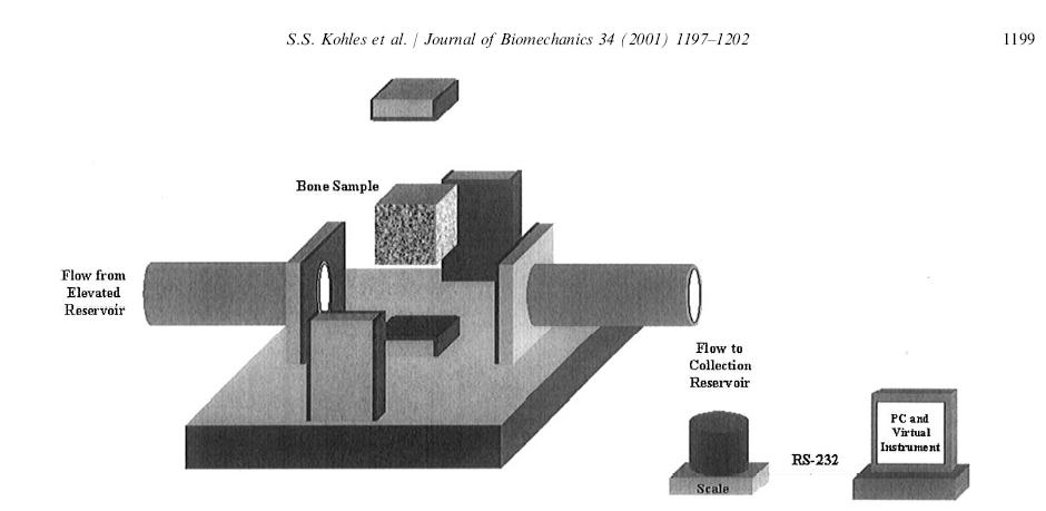
which allowed measurement of anisotropic permeability for cancellous bone. The permeability was measured by allowing water to flow from an elevation through the cancellous bone sample to a collection reservoir. By measureing fluid mass flow rate dm/dt, the specimen length L, the water viscosity m, the area of the specimen A, and the pressure gradient delta p, the permeability K could be calculated as:

      

The elasticity constants were measured from ultrasonic wave speed as:

    

Thus, using this approach, Kohles and Roberts could determine some constants for linear poroelasticity theory as applied to cancellous bone, in this case from the bovine (cow) distal femur. Results showed that, as expected, increasing elastic modulus was correlated with decreasing permeability:

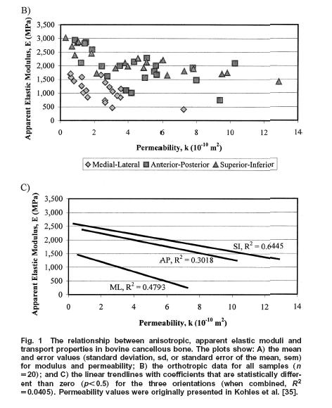
In terms of a structure-function relatonship, Kohles and Roberts plotted porosity versus both elasticity:

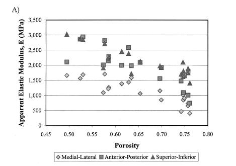
which showed a weak negative correlation, indicating that porosity was a contibutor to decreased elastic properties, but not the only contributor. They also found that increasing porosity was correlated weakly with increasing permeability:

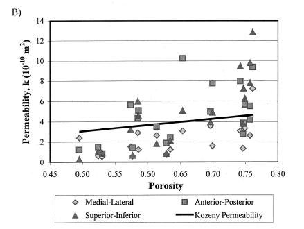
Both these structure-function results strongly suggest that other aspects of trabecular bone structure would more strongly correlate with both the elastic and permeability constants from linear poroelasticity theory, perhaps the anisotropy tensor that was used previously to correlate with elastic constants.

XI. Viscoelastic Models of Bone

Bone has also been characterized as a viscoelastic material. Iyo et al. (2004, J. Biomechanics) utilized a mechanical analog to describe the viscoelastic behavior of bovine (cow) cortical bone. The used a the following function to describe relaxation of Young's modulus:

where E0, A1, b, and g are experimental constants to be determined and t1 and t2 are characteristic relaxation times which must also be fit to data. In this case, Iyo et al. divide the response into a fast relaxation process (associated with A1) and a slow relaxation process, (associated with (1-A1)). Iyo et al. tested cortical bone specimens from bovine distal femur as shown in the following orientation:

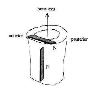
They determined the following parameters for the relaxation model for the P and N specimens:

                    Parameter:             E0 (GPa)          A1               t1 (sec)                    t2 (sec)

N                                              14.2                 .08                49                           9300000

P                                              11.6                  0.11              50                           6400000