I.          Overview

            Ligaments and tendons are soft collagenous tissues. Ligaments connect bone to bone and tendons connect muscles to bone. Ligaments and tendons play a significant role in musculoskeletal biomechanics. They represent an important area of orthopaedic treatment for which many challenges for repair remain. A good deal of these challenges have to do with restoring the normal mechanical function of these tissues. Again, as with all biological tissues, ligaments and tendons have a hierarchical structure that affects their mechanical behavior. In addition, ligaments and tendons can adapt to changes in their mechanical environment due to injury, disease or excerise. Thus, ligaments and tendons are another example of the structure-function concept and the mechanically mediated adaptation concept that permeate this biomechanics course. In this section, we will review aspects of ligament and tendon structure, function and adaptation. These notes follow very closely Chapter 6 on Structure and Function of Tendons and Ligaments from your text.

II.         Hierarchical Ligament and Tendon Structure

            We start out again emphasizing that ligaments and tendons have a hierarchical structure. One schematic of this hierarchical structure is taken from your text, and is a very famous schematic from Kasterlic:

                            

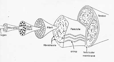
The largest structure in the above schematic is the tendon (shown) or the ligament itselt. The ligament or tendon then is split into smaller entities called fascicles. The fascicle contains the basic fibril of the ligament or tendon, and the fibroblasts, which are the biological cells that produce the ligament or tendon. There is a structural characteristic at this level that plays a significant role in the mechanics of ligaments and tendons: the crimp of the fibril. The crimp is the waviness of the fibril; we will see that this contributes significantly to the nonlinear stress strain relationship for ligaments and tendons and indeed for bascially all soft collagenous tissues.

The above schematic shows the basic common structures for ligaments and tendons. In terms of specific attributes for tendons:

TENDONS

Anatomy:

            1. Tendons contain collagen fibrils (Type I)
            2. Tendons contain a proteoglycan matrix
            3. Tendons contain fibroblasts (biological cells) that are arranged in parallel rows

Basic Functions

            1. Tendons carry tensile forces from muscle to bone
            2. They carry compressive forces when wrapped around bone like a pulley

Type I Collagen:

            1. ~86% of tendon dry weight
            2. Glycine (~33%)
            3. Proline (~15%)
            4. Hydroxyproline (~15%, almost unique to collagen, often used to identify)

Blood Supply:

            1. Vessels in perimysium (covering of tendon)
            2. Periosteal insertion
            3. surrounding tissues

LIGAMENTS

Anatomy

            1. Similar to tendon in hierarchical structure
            2. Collagen fibrils are slightly less in volume fraction and organization than tendon
            3. Higher percentage of proteoglycan matrix than tendon
            4. Fibroblasts

Blood Supply

            1. Microvascularity from insetion sites
            2. Nutrition for cell population; necessary for matrix synthesis and repair

III.       General overview of ligament and tendon mechanics

            As with all biological tissues, the hierarchical structure of ligaments and tendons has a signficant influence on their mechanical behavior. Unlike bone, however, not nearly as much quantiative structure function relationships, either experiment/statistical or analytical, have been derived for ligaments and tendons. This is for two reasons: 1) the hierarchical structure of ligaments and tendons is much more difficult to quantify than bone, and 2) ligaments and tendons exhibit both nonlinear and viscoelastic behavior even under physiologic loading, which is more difficult to analyze than the linear behavior of bone.

Nonlinear Elasticity 

           If one neglects viscoelastic behaviour, a typical stress strain curve for ligaments and tendons can be drawn as:

                          

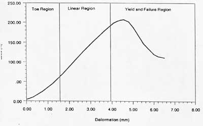
There are three major regions of the stress strain curve: 1) the toe or toe-in region, 2) the linear region and 3) the yield and failure region. In physiologic activity, most ligaments and tendons exist in the toe and somewhat in the linear region. These constitute a nonlinear stress strain curve, since the slope of the toe-in region is different from that of the linear region.

In terms of structure function relationships, the toe-in region represents "un-crimping" of the crimp in the collagen fibrils. Since it is easier to stretch out the crimp of the collagen fibrils, this part of the stress strain curve shows a relatively low stiffness. As the collagen fibrils become uncrimped, then we see that the collagen fibril backbone itself is being stretched, which gives rise to a stiffer material. As individual fibrils within the ligament or tendon begin to fail damage accumulates, stiffness is reduced and the ligament/tendons begins to fail. Thus a key concept is that the overall behavior of ligaments and tendons depends on the individual crimp structure and failure of the collagen fibrils.

A simple model illustrating the dependence of ligament/tendon nonlinear stress/strain relationships is shown below:

                         

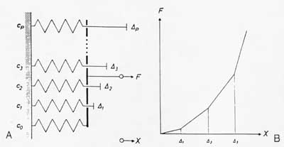
In this case, as a spring is stretched to its limit its stiffness increases. This can easily be seen if the effective ligament stiffness is modeled using the Voight model, with each fibril contributing a small part to the overall stiffness. As a fibril becomes uncrimped, its stiffness increases, increasing the overall ligament/tendon stiffness.

Viscoelasticity

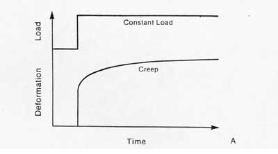
            Another important aspect of ligament/tendon behavior is viscoelasticity. Viscoelasticity indicates time dependent mechanical behavior. Thus, the relationship between stress and strain is not constant but depends on the time of displacement or load. There are two major types of behavior characteristic of viscoelasticity. The first is creep. Creep is increasing deformation under constant load. This contrasts with an elastic material which does not exhibit increase deformation no matter how long the load is applied. Creep is illustrated schematically below:

                         

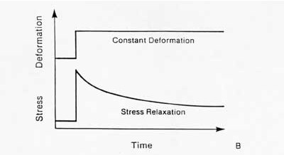
The second significant behavior is stress relaxation. This means that the stress will be reduced or will relax under a constant deformation. This behavior is illustrated below:

                                     

The other major characteristic of a viscoelastic material is hysteresis or energy dissipation. This means that if a viscoelastic material is loaded and unloaded, the unloading curve will not follow the loading curve. The difference between the two curves represents the amount of energy that is dissipated or lost during loading. An example of hysteresis is shown below:

                            

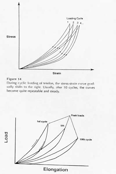
The two figures above show that the amount of hysteresis under cyclic loading is reduced and eventually the stress-strain curve becomes reproducible. This gives rise to the use of pseudo-elasticity to represent the nonlinearity of ligament/tendon stress strain behavior.

Finally, in this overview of ligament/tendon mechanics we discuss briefly experimental considerations in testing ligaments and tendons. Directly measuring ligament or tendon behavior by directly griping the specimen can lead to erroneous measurements. This is because ligaments and tendons are extremely difficulty grip firmly and often slide in the grips leading to errors in displacement measurements. A way around this difficulty is to leave the ligament attached to the bone and use optical methods and markers to measure the strain. A schematic of such a test setup from the text is shown below:

                         

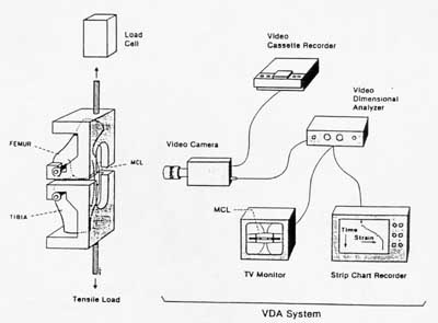
The grips are placed around the bones of the joint to give a much more secure fit. In the case of tendons, there is still a need to grip the muscle end.

IV       Modeling Ligaments and Tendons as Nonlinear Elastic Materials

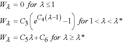
            To represent the nonlinear elastic behavior of ligaments, Weiss et al. has developed a hyperelastic model including a strain energy function. Weiss sought to represent the contributions of collagen fibers, the ground substance and the interaction between the two. The strain energy function is given below:

            

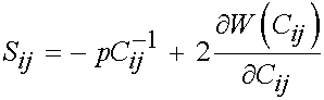
where Ii are the invariants of the right Cauchy deformation tensor. The 2nd Piola-Kirchoff stress tensor is calculated from the above strain energy function by the relationship:

            

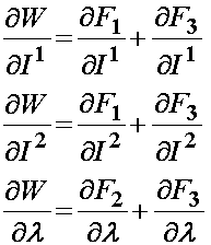
Another model described by Wiess and Gardiner (2001, Crit. Rev. Biomedical Engineering) described ligament behavior as nonlinear elastic using a transversely isotropic strain energy function. This was written as:

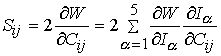
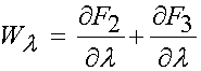
where F1 represents the contribution of the isotropic ground matrix, F2 represents the contribution of the collagen fibers, and F3 represents the interaction between the collagen fibers and the matrix. The ligaments are also assumed to be incompressible due to the presence of water in the matrix. Recall that the general form of the 2nd Piola Kirchoff stress for an incompressible isotropic hyperelastic material is:

This may be modified to account for transverse isotropy as:

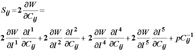
Since Weiss did not include the 5th invariant, the final form of the 2nd PK stress for a transversely isotropic material would be:

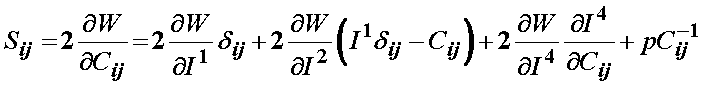
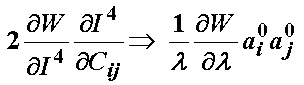
The term associated with the I4 invariant can be written recognizing it depends on the stretch function l as:

Thus, the total 2nd Piola-Kirchoff stress for the ligament modeled using the transversely isotropic strain energy function is:

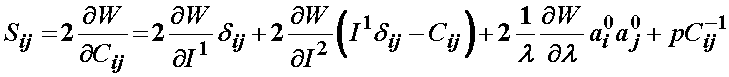
Based on the definition of the strain energy function consisting of three components F1, F2, and F3, the 2nd PK stress is defined as:

For the isotropic ground substance strain energy function, a Mooney-Rivlin type model was proposed:

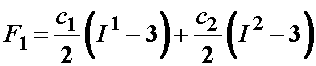
No strain energy function was proposed for F2 because this term characterized the ligament ground substance under shear for which a test was not performed. For the collagen representation, which was characterized as follows:

It was noted that collagen fibrils do not sustain compression, and that the tensile behavior follows the classic stress-strain curve with toe-in region followed by a linear region. This was written as:

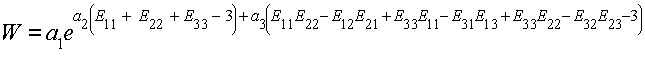
Two recent papers have used the more common isotropic form of the strain energy function for analyzing stress and strain in anteior cruciate ligamens. The first was by Hirokawa and Tsuruno in Medical Engineering and Physics (1997), 19:637-651. They used a strain energy function commonly used for rubber like materials, also called a Mooney-Rivlin strain energy function. It is given below:

           

where I1 and I2 are invariants of the right Cauchy Deformation tensor. There are defined as:

            

           

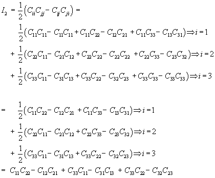
 Thus, we can rewrite W using the explicit form of the invariants I1 and I2 as:

                  

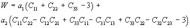
where a1 and a2 are constants to be determined experimentally.   Let us now assume that the 11 direction lies along the length of the ligament and we would like to determine the stress/strain curve along that direction. We must first take the derivative of W with respect to E11.  First we know the relatonship between E11 and C11 is:

          

The derivative can be taken using the chain rule as:

             

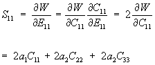
We can rewrite the above equation in terms of E using the general equation relating E to C (the right Cauchy Deformation Tensor):

            

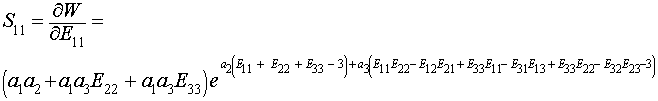
This gives S11 in terms of E as:

           

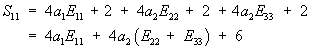
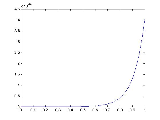
To plot S11 vs. E11, we need to know E22 and E33.   We will assume for our case that they are 0. In addition, we need to know the material constants a1 and a2. Hirokawa and Tsuruno report these to be 1.687 and 0.106 (kg/cm2), respectively, which, given that 1 kg/cm2 is equivalent ot 98 KPa, gives constants of 165.3 KPa and 5.88KPa. We can make the stress strain plot in MATLAB for s11 vs. e11 (assuming all other strains are zero) using the following commands:

e11 = (0:99)/99;
for i = 1:100
s11(i) = 4.*165.3*e11(i)+6.;
end
plot(e11,s11)
xlabel('strain E11')
ylabel('stress S11 (KPa)')

This yields the following linear relation between the 2nd Piola-Kirchoff stress and Green-Lagrange strain:

A second paper utilizing an isotropic strain energy function to model human anterior cruciate ligament behavior was published by Song et al. in the Journal of Biomechanics, 37:383-390, 2004. Song et al. used a strain energy function that was originally proposed by Veronda and Westmann for skin in 1970 (Veronda and Westmann, J. Biomechanics, 3:111-124, 1970). This strain energy function is given below:

          

where I1 and I2 are the 1st and 2nd invariants of the Green-Lagrange strain tensor, e is the exponential function, and a1,a2,a3 are constants to be experimentally determined.   Based on our previous expansion of the invariants, we write the strain energy function directly in terms of the Green-Lagrange strain tensor components as:

         

To calculate the S11 component of the 2nd Piola-Kirchoff stress, we again take the derivative of W with respect to E11:

         

We can then plot a stress-strain curve using the values for the experimental coefficients a1,a2 and a3. If we assume that all strains except E11 are zero due to the test set up, we can write the following MATLAB commands to plot the stress versus strain curve:

e11 = (0:99)/99;
for i = 1:100
s11(i)=0.26*11.35*exp(11.35*e11(i)-11.35*3.)
end
plot(e11,s11)

As we can see, for this large of strain we only see significant nonlinear behavior for strains well over 50%. For strains more in the physiologic range of ligaments, say up to 10% strain we have:

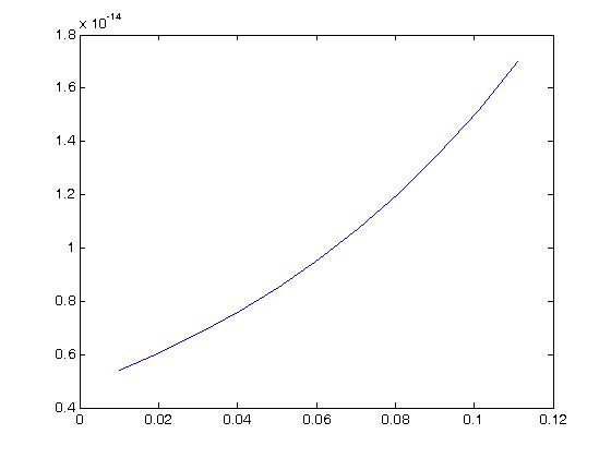
which we can see has a more linear behavior.

VI.        Modeling Ligaments as Viscoelastic Materials

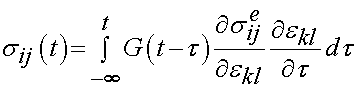
            As ligaments and tendons exhibit time dependent behavior, a number of studies have modeled ligaments and tendons using viscoelastcity, especially QLV theory. Weiss and Gardiner provided one form of the above equation is the QLV implementation, which is written for the 2nd PK stress tensor as:

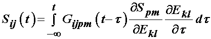
it is generally assumed that the relaxation function is the same in all directions, which means that the stress relaxation tensor is actually a scalar and the above is written as:

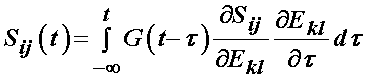
with the reduced relaxation function being:

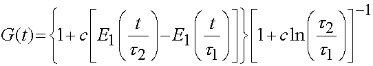
It has been determined that the consant c has the greatest influence on the viscous behavior and that the time constants t1 and t2 determine fast and slow viscous behavior. For purposes of finite element analysis, Puso and Weiss approximated the reduced realxation function as:

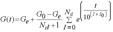
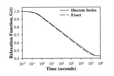
where Ge are the equilibrium modulus, G0 is the initial modulus, Nd is the number of decades on a log scale, and 10^I0 is the lowest discernible relaxation time. Puso and Weiss showed that the discrete represented the analytical form of the stress relaxation function very well as shown below:

A recent example of where QLV theory was applied to model the mechanical behavior of normal versus healing ligaments was provided by Abramowitch et al. (2004) using a coefficient fitting routine developed by Abramowitch and Wu (2004). They determined QLV parameters for both normal and healing Medical Collateral Ligaments (MCL) in a goal model for 12 weeks post-injury. The basic formulation again begins with the fundamental QLV theory representing stress as a reduced relaxation function times an instanttaneous elastic response se:

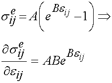
We again use the same reduced relaxation function as given above. The instant elastic response is given as:

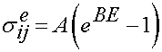
where A and B are constants and E is the uniaxial value of the large strain tensor.

In Abramowitch and Wu's approach, the reduced relaxation function and instantaneous elastic response are substituted into the convolution history integral that gives stress as a function of time:

where the quantity:

represents the strain history to which the tissue is subjected. If we take the derivative of the instant elastic response with respect to the strain we get:

To calculate material constants, we need to specify a strain history to which the material will be subjected. As noted in the section on viscoelasticity, we will subject the material to a step strain test, where the strain is ramped up and then held constant. Also noted in that section was the fact that no testing machine can instantaneously apply strain. Therefore, the strain is applied over a finite time and looks like the following:

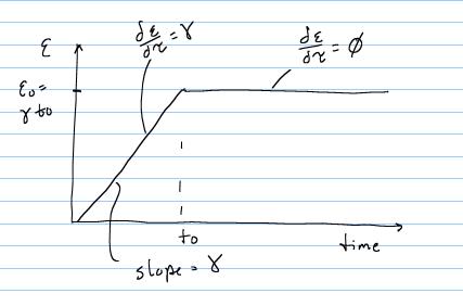
From t = 0 to t = t0, there is constant linear increase in strain with slope g, and the total strain at any time during the ramp is simply gt. Thus, for this time frame the strain time history is:

Over the time period t = t0 to the end of the testing period, the strain level is held constant and thus:

Thus in the ramp period where t > 0 and t < t0, we have the stress as:

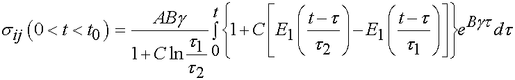
For the time period t > t0 we have the following:

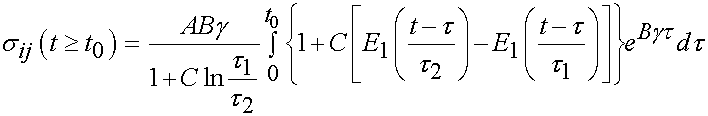
The integral only extends to t0 because the derivative of strain with respect to time is zero after t0. To fit the constants an optimization scheme called a least squares fit is used. In this case, the objective function is the model as shown above minus the actual experimenal data squared. For the time dependent case, a two part objective is used, one least squares fit for the ramp zone and one for the constant strain zone. The objective function for the least squares case is:

In this case, the experimental constants are updated by the optimization algorithm to until the objective function is minimized. Using this approach, Abramowitch et al. studied the difference in mechanical function as characterized by QLV for normal and healing medial collateral ligaments (MCL). The hypothesis was that healing ligaments have lower instantaneous modulus and exhibit more stress relaxation than normal ligaments. The experimental model was a goat model in which the MCL was ruptured and then the ends were reapproximated but not sutured. Normal had an operation with exposure but the ligament was not touched. Animals were sacrificed at 12 weeks and a femur MCL tibia complex was used to test the ligaments. Results did in fact indicate that healing ligaments had a lower instantaneous modulus and a higher degree of stress relaxation compared to normal ligaments. In this case, the structure is qualitatively described as healing versus normal, and we see the outcome in a structural measure. A typical stress relaxation curve for normal and healing ligaments is shown below, were the boxes are experimental data and the lines are the QLV curve fit:

VII.        Structure-Function in Ligaments/Tendons: Aging Effects

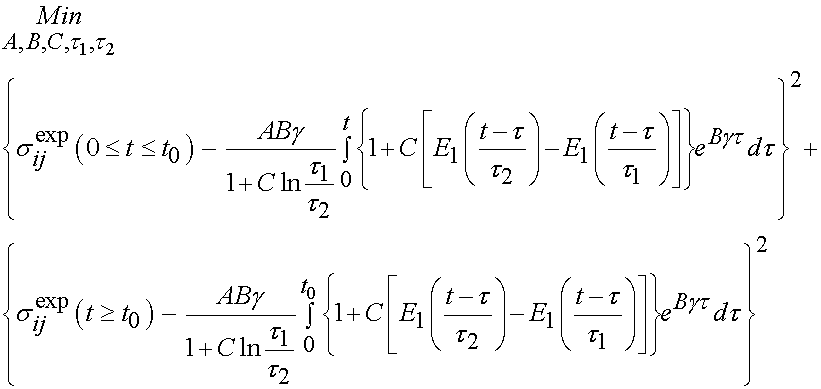
            Much of our knowledge of structure-function relationships for ligaments and tendons is empirical and not strictly quantiative as with bone, for reasons we touched upon earlier. Most studies on structure-function relationships in ligaments and tendons come from comparisons of mechanical properties and histology/biochemistry of ligaments and tendons from young versus old animals. For example, in rat tail tendons, the diameter of collagen fibrils increase during age from skeletally immature to mature animals. There is a corresponding increase in the ultimate tensile strength of the tendons. In a study of New Zealand white rabbits at 1.5 months, 4-5 months, 6-7 months, and 12-15 months, it was determined that the stiffness and strength of both the mid-ligament substance and the ligament bone attachment increased with increasing maturity in the femur-mcl-tibia complex (FMTC). The change in ligament attachment strength was due to rapid remodeling of bone near the insertion site in younger animals. A schematic drawing showing this change in material properties with age is shown below:

                            

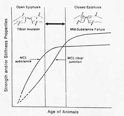
You can see from this graph that as the strength of the ligament insertion increases, failures change from being avulsion failures to being mid-substance failures. A quantitative example of the increase in mechanical properties with maturity is shown in the graph from your text below:

                            

            While increasing age from child to adult also increases the mechanical properties of ligaments and tendons, further increasing age from young adulthood decreases the properties of ligaments and tendons. One study found that structural properties of the FATC (femur-acl-tibia complex) decreased by 2-3 times for older versus younger adult knees. Structural properties refer to the stiffness of the ligament in the bone-ligament-bone testing mode when it is not calculated using normalized stress and strain values, ie force vs displacement.
Woo and colleagues tested FATC from young cadaver knees with an average age of 35 and older cadaver knees with an age of 76. They found that the linear structural stiffness of the ACL decreased both when tested at 30 degrees of knee flexion and when tested along the axis of the ligament complex. The structural stiffness in the ligament axis averaged 183 N/mm for the younger group but only 158 N/mm for the older group. Tests under flexion were 150 N/mm and 129 N/mm for the younger and older group respectively. In addition, more specimens in the older group suffered avulsion failures than the younger group.

VI.       Mechanically Mediated Ligament and Tendon Adaptation: Immobilization versus Exercise

            Ligaments and tendons are adapted in response to changes in mechanical stiffness. The changes in ligaments and tendons generally occur more slowly than adaptation in bone, because ligaments and tendons have less vascular supply. Again, our knowledge of how mechanical stimulus mediates ligament and tendon structure is more empirical and less rigorous than that for bone. Most of our knowledge comes from two extremes in mechanical stimulus: immobilization and exercise.

            Immoblization of a joint for a long period of time leads to significant changes in joint structure and function, including decreased range of motion for the joint. The affects of both ligaments and tendons can be severe. Woo et al. studied rabbit knees in the following experimental groups:

1. 9 weeks immobilization
2. 12 weeks immobilization
3. 9 weeks immobilization, then 9 weeks active
4. 12 weeks immoblization, then 9 weeks active

9 weeks of immoblization led to a 69% decrease in ultimate load and an 82% decrease in energy to failure. After 12 weeks of immoblization led to a 71% decrease in ultimate load. Affects on the stress strain curve from Woo are shown below:

                        

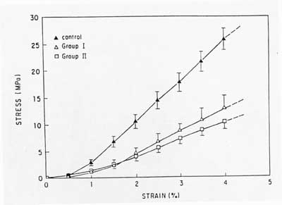
If the rabbits became active, there was an increase in stiffness and strength almost back to the level of controls.

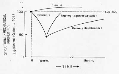
Corresponding to the reduction in mechanical properties, there is a reduction in the ligament structure. During immobilization, the cross sectional area of the ACL is reduced. This implies a loss of collagen fibrils as well as a loss of glycosaminoglycans that form the ground substance of the ligament. In addition, the may be alterations in collagen fibril orientation that reduce properties. Upon remoblization, it appears that the mechanical properties of the ligament are gained back first, followed by the structural properties. This indicates that structural loss at the ligament insertion site may take longer to be removed that changes in ligament substance.

Excercise and increased load on tendons and ligaments is believed to alter their structural makeup and lead to increased mechanical properties, although experimental data is far from conclusive. Woo et al studied the affect of exercise on swine digital tendons and the FMTC. Animals were run on a track at speeds of 6 to 8 km/hr for an average of 40km/week for 3 months and 12 months.. A sedentary group was used as a control. The short term group showed no significant changes in mechanical properties for either the tendons or the FMTC. There was an increase in cross-sectional area of the tendon as well as a 22% increase in tensile strength. For the FMTC, however, there was little change in most mechanical properties, although there was a significant increase in maximum load to failure when normalized by animal weight. Another study in dogs also found higher ultimate load to body strength ratios for the FMTC. Woo put the findings on immobilization and exercise together in a graph showing how changes in mechanical load may alter ligament/tendon structure, in a statement he characterized as Wolff's law for ligaments/tendons. This hypothesis from the text is shown below:

                         

As you can see, immobilization has a more rapid and substantial affect on mechanical properties than does increased load from exercise. This is in some ways similar to Frosts theory on adult bone adaptation, where he believed it was difficult to achieve substantial increase in bone structure through mechanical loading unless damaged was caused, but that losses in bone mass were realized quite readily when loads were significantly reduced as in immobilization. The same can be seen in the above graph for ligaments and tendons.

VII       Mechanics of and Mechanical Affects on Healing Tendons/Ligaments

            One of the most important topics in mechanically mediated ligament and tendon adaptation is the effect of mechanical stimulus on ligament and tendon repair. Ligament and tendon repair are a critical area of orthopaedic surgery, especially in sports medicine. Important issues in ligament and tendon repair are how the ligament should be repaired, if applying mechanical load hinders or helps repair, and when repair has progressed to the point where complete load bearing is possible.

            In the case of tendons, which glide within a sheath, the introduction of passive motion for healing and repaired tendons is believed to be important because it prevents adhesion between the sheath and tendons that restricts motion. In one study, the flexor tendons of skeletally mature dogs were lacerated and then repaired. There were three experimental groups: 1) compete immobilization, 2) delayed mobilization and 3) early passive motion. The results indicated that tendon strength and motion increased more quickly for the early passive motion group than for the other two groups.

The relationship between mobilization following repair and alterations of ligament structure and function is complex, depending on how long the ligament is immobilized following repair. In a study of Medial Collateral Ligament (MCL) repair, MCL were lacerated and then repaired. In one group, the MCL was not repaired, but it was immobilized. In the second group, the MCL was repaired and immobilized for three weeks while in the third group immoblization lasted for 6 weeks. Suprisingly, the group without repair that was immobilized early showed the best gain in strength over time. This reflected changes in the structural makeup of the ligament. The amount of type I vs. type III collagen (type III collagen is a type of collagen associated with wound healing) was closer to normal for the early mobilized ligament without repair. The change in strength over time is shown in the figure below (group 1 is the early mobilization without repair, group 2 is repair with 3 week immobilization and group 3 is repair with 6 week immobilization):

                      

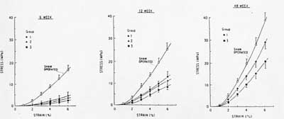
These results demonstrate two basic concepts: 1) in a confirmation of tissue structure function relationships, the stiffness and strength of healing ligaments correlates with the type and amount of collagen fibrils present, and 2) that mechanical stimulus has a significant affect on ligament structure.